Interpolation is used in financial analysis to estimate missing values.
Click the image for a detailed view
Download Practice Workbook
What Is Interpolation?
Interpolation is a mathematical technique used to estimate values within a set of known data points. It fills gaps between observed data points by assuming a smooth or linear relationship between them. Interpolation can be linear or non-linear, depending on the data nature and accuracy.
How to Do Linear Interpolation for Linear Dataset in Excel?
If your dataset is linear, you can implement a linear interpolation method. The image below displays a set of formulas that you can use to perform linear interpolation on a linear set of data.
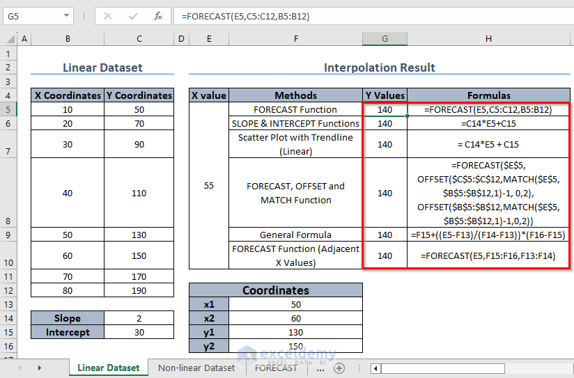
Click the image for a detailed view
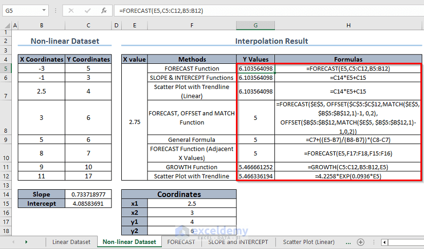
How to Do Linear Interpolation for Non-linear Dataset in Excel? (Taking All X & Y Values into Consideration)
If your dataset is non-linear, you may get different interpolation results if you follow different methods. You can perform linear interpolation either by taking all X & Y values or only the adjacent X & Y values.
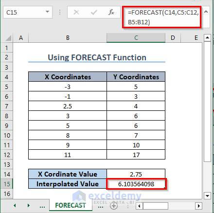
1. Using the FORECAST Function
- Use the following formula in C15:
=FORECAST(C14,C5:C12,B5:B12)- Press Enter.
2. Using SLOPE and INTERCEPT Functions
Slope = SLOPE(C5:C12,B5:B12)
Intercept = INTERCEPT(C5:C12,B5:B12)
- In C15, enter the following formula:
=E6*C14+E8- Press Enter.
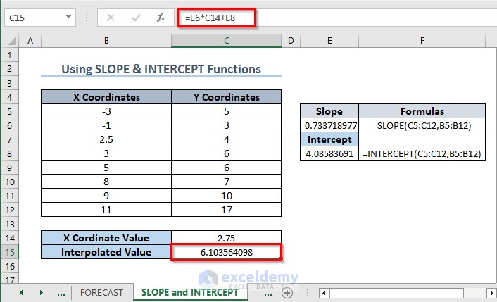
(This method follows the straight line equation, y = mx + c)
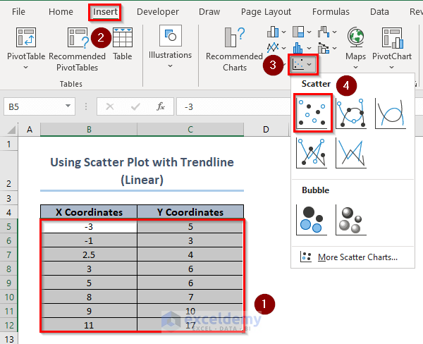
3. Using the Excel Scatter Plot (Linear Trendline)
- Select the X and Y coordinate values and click Insert >> Charts >> Scatter.
- Click Chart Elements. Check Trendline. Uncheck Gridlines.
- Change the chart title.
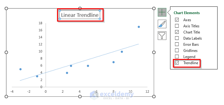
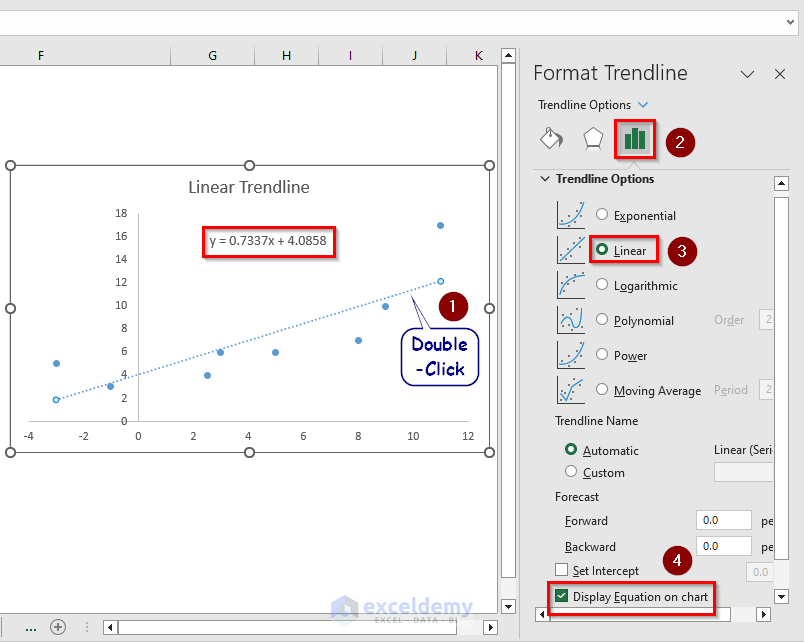
- Double-click Trendline.
- Select Trendline Options >> Linear >> Display Equation on Chart.
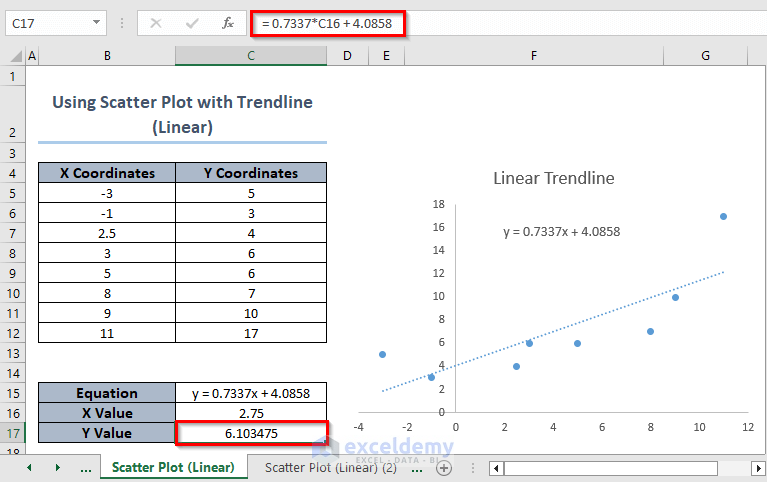
The linear equation is visible. You can enter an X value and get the corresponding Y value.
Click the image for a detailed view
- In C17, enter the following formula:
=0.7337*C16 + 4.0858- Press Enter.
How to Do Linear Interpolation in a Non-linear Dataset in Excel? (Taking Adjacent X & Y Values into Consideration)
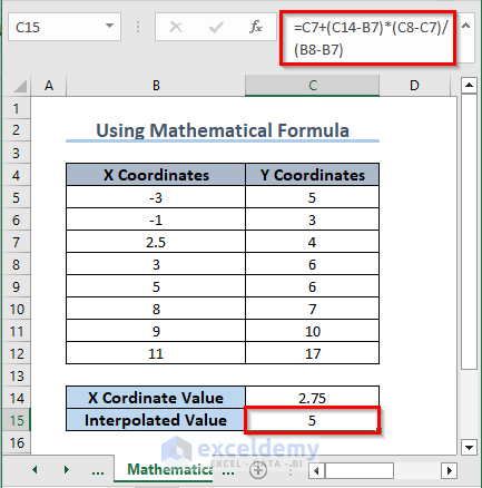
1. Using a General Mathematical Interpolation Formula
- Use the following formula in C15:
=C7+(C14-B7)*(C8-C7)/(B8-B7)
- Press Enter.
2. Using the FORECAST Function
The FORECAST function is used before interpolation. It takes all adjacent X and Y values as input.
To find the adjacent X, and Y values, use a combination of the INDEX and MATCH functions or the XLOOKUP function.
Formulas for INDEX & MATCH
- For X1 :
=INDEX(B5:B12,MATCH(C14,B5:B12,1)) - For X2 :
=INDEX(B5:B12,MATCH(C14,B5:B12,1)+1) - For Y1 :
=INDEX(C5:C12,MATCH(C14,B5:B12,1)) - For Y2 :
=INDEX(C5:C12,MATCH(C14,B5:B12,1)+1)
Formulas for XLOOKUP
- For X1 :
=XLOOKUP($C$14, B5:B12,B5:B12,,-1,1) - For X2 :
=XLOOKUP($C$14, B6:B13,B6:B13,,1,1) - For Y1 :
=XLOOKUP($C$14, B5:B12,C5:C12,,-1,1) - For Y2 :
=XLOOKUP($C$14, B5:B12,C5:C12,,1,1)
- In C15, enter the following formula:
=FORECAST(C14,F8:F9,F6:F7)- Press Enter.

Click the image for a detailed view
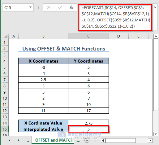
3. Combining the FORECAST, OFFSET, and MATCH Functions
- In C15, enter the following formula:
=FORECAST($C$14, OFFSET($C$5:$C$12,MATCH($C$14, $B$5:$B$12,1)-1, 0,2), OFFSET($B$5:$B$12,MATCH($C$14, $B$5:$B$12,1)-1,0,2))- Press Enter.
Formula Breakdown
- MATCH($C$14, $B$5:$B$12, 1): Finds the position of the largest value less than or equal to the lookup value in B5:B12.
- OFFSET($B$5:$B$12, MATCH($C$14, $B$5:$B$12, 1)-1, 0, 2): Creates a new range by shifting B5:B12 by the number of rows specified by the result of the MATCH function minus 1, with a resulting range height of 2 rows.
- OFFSET($C$5:$C$12, MATCH($C$14, $B$5:$B$12, 1)-1, 0, 2): Creates a new range by shifting C5:C12 by the number of rows specified by the result of the MATCH function minus 1, with a resulting range height of 2 rows.
- FORECAST($C$14, OFFSET($C$5:$C$12, MATCH($C$14, $B$5:$B$12, 1)-1, 0, 2), OFFSET($B$5:$B$12, MATCH($C$14, $B$5:$B$12, 1)-1, 0, 2)): Performs linear interpolation using the FORECAST function, using the value in C14 as the X value and interpolating between two adjacent data points based on their corresponding X and Y values (shifted using OFFSET).
How to Do Non-linear Interpolation in Excel?
Non-linear interpolation returns more accurate results.
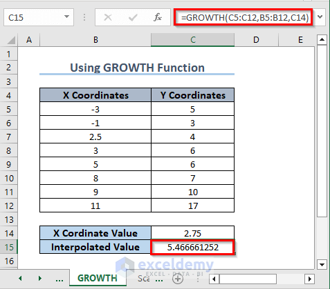
How to Do Non-linear Interpolation Using the GROWTH Function?
Use the GROWTH function.
- In C15, enter the following formula:
=GROWTH(C5:C12,B5:B12,C14)- Press Enter.
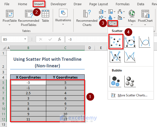
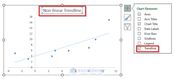
How to Do Non-linear Interpolation Using a Scatter Plot with a Trendline?
- Select the X and Y coordinate values and click Insert >> Charts >> Scatter.
- Click Chart Elements.
- Check Trendline.
- Uncheck Gridlines.
- Change the chart title.
- Double-click Trendline.
- Select Trendline Options >> Exponential >> Display Equation on Chart.
The linear equation is visible. Enter the X value and get the corresponding Y value.
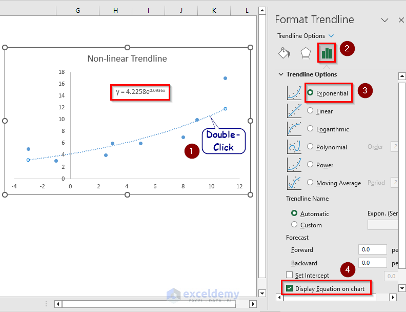
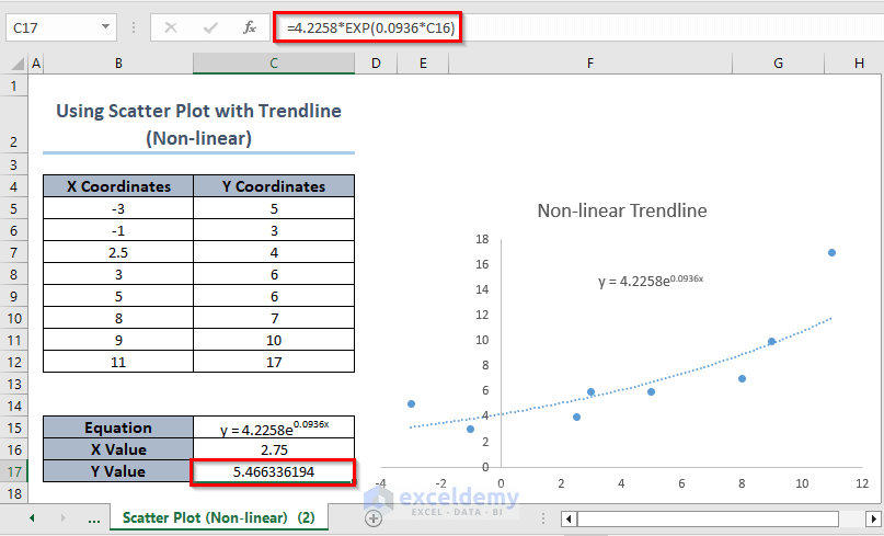
- In C17, enter the following formula:
=4.2258*EXP(0.0936*C16)- Press Enter.
Click the image for a detailed view
Practical Examples of Interpolation in Excel
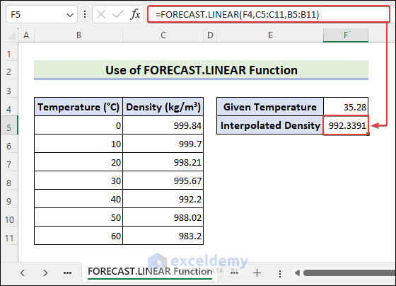
How to Use the FORECAST.LINEAR Function to find Density?
Use FORECAST.LINEAR function. It determines a prediction using a straight line that fits known data.
- Select F5 >> enter the formula >> press Enter.
=FORECAST.LINEAR(F4,C5:C11,B5:B11)
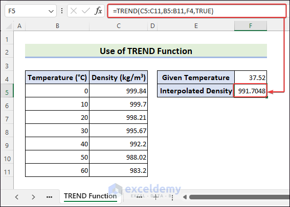
How to Apply the TREND Function to Get Interpolated Density?
Apply the TREND function to get interpolated density.
- Select F5 >> use the following formula >> press Enter.
=TREND(C5:C11,B5:B11,F4,TRUE)
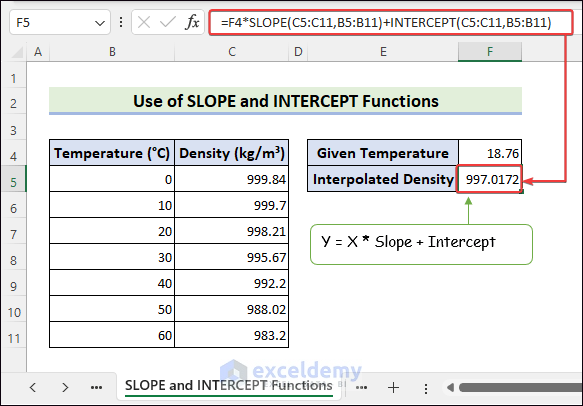
How to Do Interpolation With the SLOPE and INTERCEPT Functions?
The SLOPE function finds the slope of a straight line. The INTERCEPT function calculates the point where the line crosses the y-axis.
- Select F5 >> enter the following formula >> press Enter.
=F4*SLOPE(C5:C11,B5:B11)+INTERCEPT(C5:C11,B5:B11)
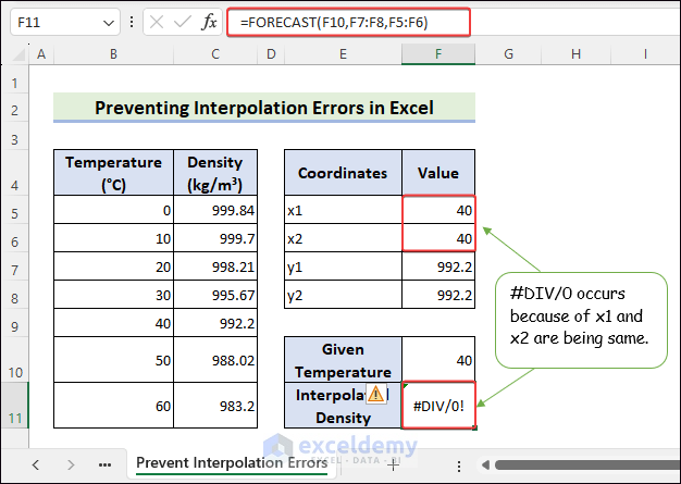
How to Prevent Interpolation Errors in Excel?
#DIV/0 is often displayed because x1 and x2 are the same. To prevent this error:
- Select F11 >>use the formula >> press Enter to see #DIV/0.
=FORECAST(F10,F7:F8,F5:F6)
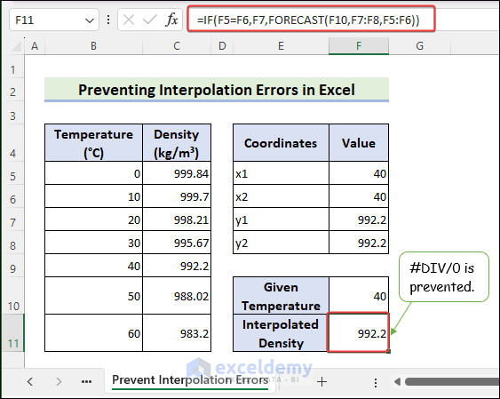
Improve the formula.
- Select F11 >> enter the following formula >> press Enter.
=IF(F5=F6,F7,FORECAST(F10,F7:F8,F5:F6))
No #DIV/0 will be displayed.
What Are the Things to Keep in Mind?
- Make sure your data is organized in columns or rows, with the independent variable (X) values in one column and the dependent variable (Y) values in another column.
- Ensure that your X values are sorted in ascending order. If your data is not sorted, the interpolation results may be incorrect.
- Make sure there are no duplicate X values in your dataset. Excel’s interpolation functions rely on unique X values.
Frequently Asked Questions
1. Is there an interpolation function in Excel?
Answer: Yes, Excel provides several functions that can be used for interpolation. The most commonly used function for linear interpolation is the FORECAST function. For non-linear interpolation, Excel does not have a built-in function, but you can use other functions like TREND, GROWTH, or LINEST to perform various types of curve fitting and extrapolation.
2. What are the differences between extrapolation and interpolation?
Answer: Interpolation is the technique of estimating values within the range of known data points.
Extrapolation involves estimating values beyond the range of known data points. It extends the trend or relationship observed to predict values outside the range.
3. Is Interpolated data a reliable source of information?
Answer: The reliability of interpolated data depends on the quality of the original data and the appropriateness of the interpolation method.
Excel Interpolation: Knowledge Hub
- How to Interpolate Missing Data in Excel
- How to Do Linear Interpolation in Excel
- How to Do VLOOKUP and Interpolate in Excel
- How to Interpolate Between Two Values in Excel
- How to Do Interpolation with GROWTH & TREND Functions in Excel
- How to Use Non Linear Interpolation in Excel
- How to Interpolate in Excel Graph
- Do 2D Interpolation in Excel
- 3D Interpolation in Excel
- Linear Interpolation Excel VBA
- Calculate Logarithmic Interpolation
- Perform Exponential Interpolation
- Do Polynomial Interpolation
- Apply Cubic Spline Interpolation
- Interpolate Time Series
- Perform Bilinear Interpolation
<< Go Back to Excel for Statistics | Learn Excel
Get FREE Advanced Excel Exercises with Solutions!
