How to Do Polynomial Interpolation in Excel (With Easy Steps)

What Is Interpolation?

Interpolation means predicting a value between two specific given data points using the dataset. Data can be linear or nonlinear and according to that, the methods for interpolation also change.

Polynomial Interpolation in Excel: Step-by-Step Procedures

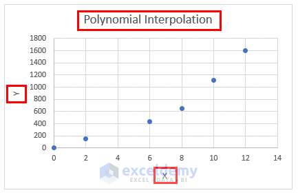
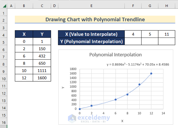
We have a sample dataset containing the values of X and Y, where Y=F(X). We will illustrate how to polynomially interpolate the value of Y from the given value of X by drawing a scatter chart in Excel.

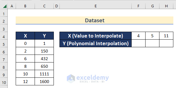
Dataset for Doing Polynomial Interpolation in Excel

Step 1 – Draw Scatter Chart

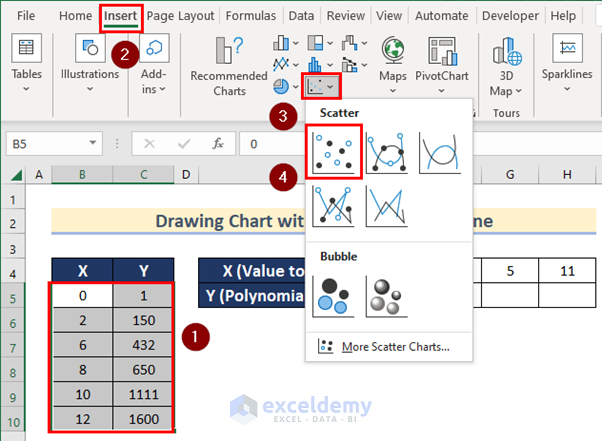
You have to insert a scatter chart to do polynomial interpolation in Excel.

Select cell range B5:C10.
Go to the Insert tab >> click on Insert Scatter or Bubble Chart >> select Scatter chart.

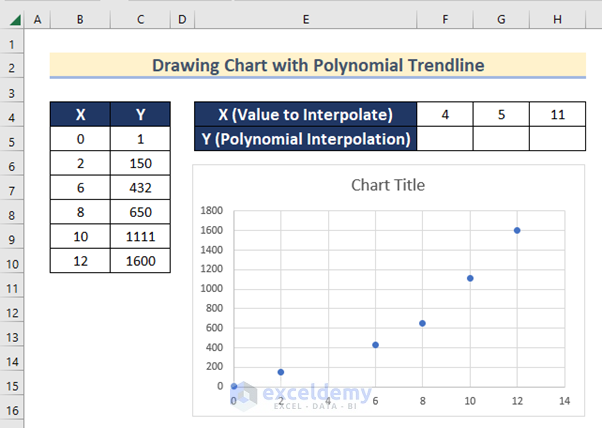
A Scatter Plot will be inserted.

Click on the “+” sign to open Chart Elements.
Check the Axis Titles option.

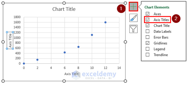
Select the titles and change the Axis and Chart Titles.

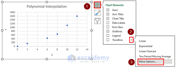
Step 2 – Add Polynomial Trendline

We will add Trendline in the Scatter plot to find the equation to interpolate data in Excel.

Click on the “+” sign to open Chart Elements.
Click on the sign beside the Trendline option.
Click on More Options.

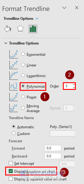
The Format Trendline toolbox will open.
Select the Polynomial option and insert Order of the polynomial.
Check the Display Equation on chart option.

It will add a polynomial trendline with the equation in the chart.

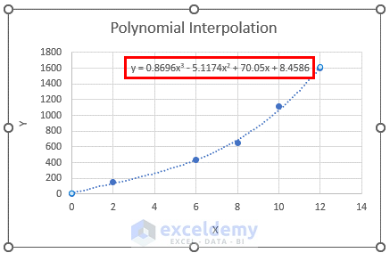
You can drag the position of the equation and make it more visible if you want.

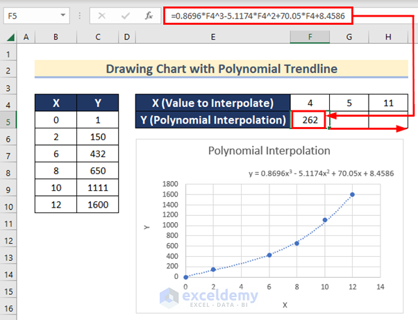
Step 3 – Find & Use Equation Found from Trendline

We will use the equation we found from the trendline to do polynomial interpolation of the data.

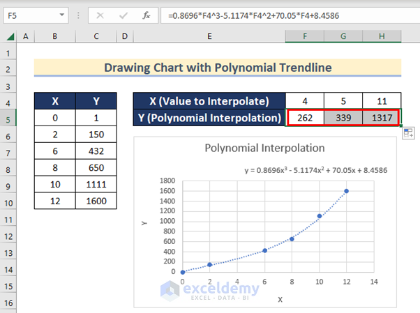
Enter the following formula which we found from the polynomial trendline in cell F5.

=0.8696*F4^3-5.1174*F4^2+70.05*F4+8.4586

Press Enter and drag right the Fill Handle tool to AutoFill the formula for the rest of the cells.

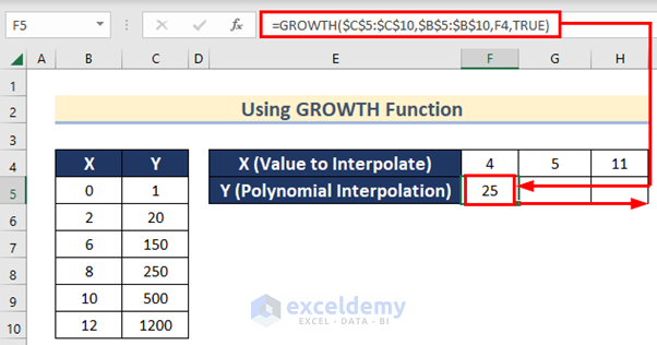
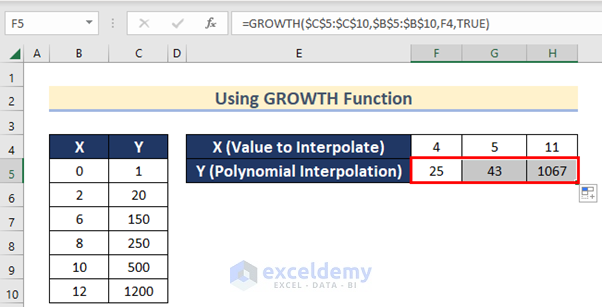
How to Perform Exponential Interpolation using the GROWTH function in Excel

The GROWTH function can predict the exponential growth of data. It uses the following equation to interpolate data.

y=b*e^x

b is the y-intercept of the curve.

To use this function to interpolate your data,

Enter the following formula in cell F5 and press Enter.

=GROWTH($C$5:$C$10,$B$5:$B$10,F4,TRUE)

Drag right the Fill Handle tool to AutoFill the formula for the rest of the cells.

In the GROWTH function, we inserted cell range C5:C10 as known_ys, cell range B5:B10 as known_xs, Cell F4 as new_xs and TRUE as const.

Things to Remember

You should check the pattern of your data (linear or nonlinear) before interpolating your data.
You can use the FORECAST & TREND functions if your data is linear.
Polynomial Interpolation is used to interpolate nonlinear data.

Download Practice Workbook

Doing Polynomial Interpolation.xlsx

<< Go Back to Excel Interpolation | Excel for Statistics | Learn Excel

Get FREE Advanced Excel Exercises with Solutions!