Introduction to The TREND Function
The TREND function calculates the values of a given set of X and Y variables and returns additional Y-values by using the least square method based on a new set of X-values along with a linear trend line.
- Syntax
=TREND(known_y’s, [known_x’s], [new_x’s], [const])
- Arguments Description
| Argument | Required/ Optional | Description |
|---|---|---|
| known_y’s | Required | A set of dependent y-values that is already known from the relationship of y = mx + b. Here,
|
| known_x’s | Optional | One or more sets of independent x-values that is already known from the relationship of y = mx + b.
|
| new_x’s | Optional | One or more sets of new x-values for which the TREND function calculates the corresponding y-values.
|
| const | Optional | A logical value specifying how the constant value b from the equation of y = mx + b should be calculated.
|
- Return Value
Calculated Y-values along with a linear trend line.
Using the TREND Function in Excel: 3 Examples
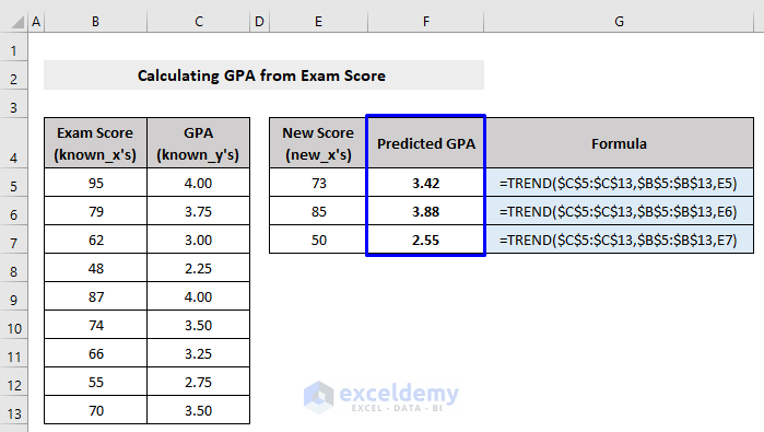
Example 1 – Calculating GPA from Exam Scores with The TREND Function
Consider the following example, where we will return the Predicted GPA of the New Score in the right table based on the Exam Score and GPA given in the left table.
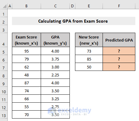
Steps:
- Pick a cell to store the result (in our case, it is cell F5).
- Insert the following formula:
=TREND($C$5:$C$13,$B$5:$B$13,E5)- Press Enter.
- AutoFill the column.
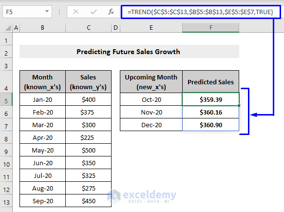
Example 2 – Predicting the Future Value with the TREND Function
We will predict future sales based on monthly sales value. We have sales value from Jan-20 to Sep-20, and with the TREND function, we will predict the sales from Oct-20 to Dec-20.
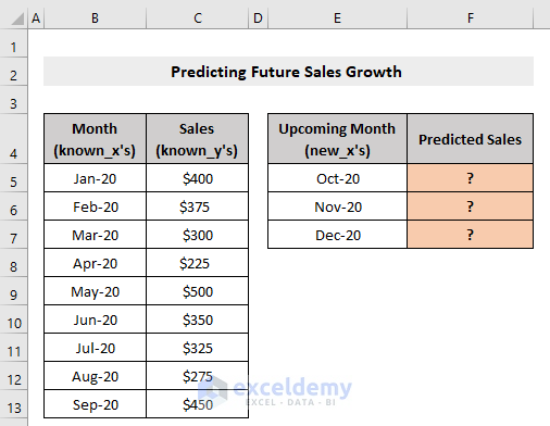
Steps:
- Pick a cell to store the result (in our case, it is cell F5).
- Insert the following formula:
=TREND($C$5:$C$13,$B$5:$B$13,$E$5:$E$7,TRUE)- Press Enter.
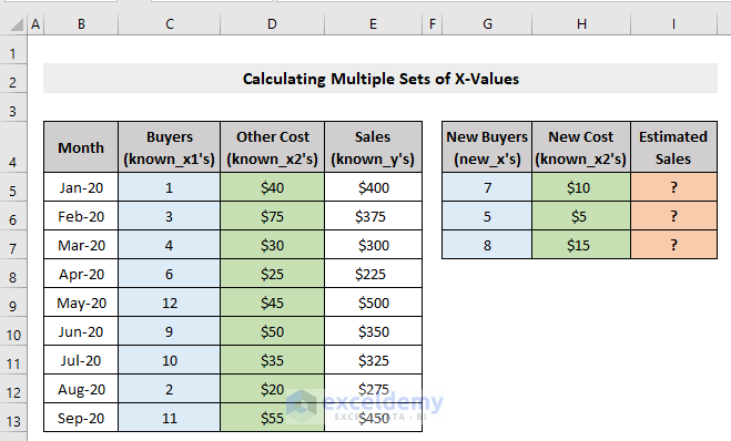
Example 3 – Utilizing Excel’s TREND Function for Multiple Sets of X-Values
We have more than one independent variables (Buyers and Other Cost in the first table). We want to calculate the Estimated Sales based on different x-values (New Buyers and New Cost in the right table).
Steps:
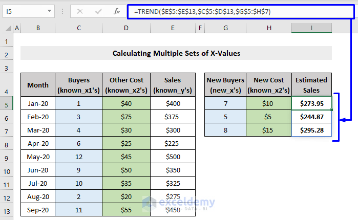
- Pick a cell to store the result (in our case, it is cell I5).
- Insert the following formula:
=TREND($E$5:$E$13,$C$5:$D$13,$G$5:$H$7)The arrays for the x-values in the formula are both 2-dimensional (C:D and G:H)
- Press Enter.
Things to Remember
- The known values – known_x’s, known_y’s – need to be linear data. Otherwise, the predicted values could be inaccurate.
- When the given values of X, Y, and new X are non-numeric, and when the const argument is not a Boolean value (TRUE or FALSE), the TREND function throws #VALUE! error.
- If the known X and Y arrays have different lengths, the TREND function returns the #REF error.
Download the Practice Workbook
<< Go Back to Excel Functions | Learn Excel
Get FREE Advanced Excel Exercises with Solutions!
