This is an overview:
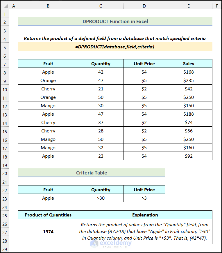
The DPRODUCT Function in Excel
Syntax:
=DPRODUCT(database,field,criteria)Arguments:
| Argument | Required/Optional | Explanation |
|---|---|---|
| database | Required | The range of cells in the database. The first row should be the column header. |
| field | Required | Defines the column from which values are extracted. It can be entered as Column Label, Column Index Number, or Cell Reference. |
| criteria | Required | The range of cells containing the criteria enlisted in them. The first row should be the column header. |
Return Value:
- Returns the product of a defined field from a database that matches specified criteria.
Remarks:
- Leave at least one row with data below the column headers.
- To perform an operation on an entire column, insert a blank row below the column header in the criteria table.
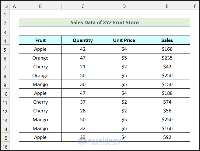
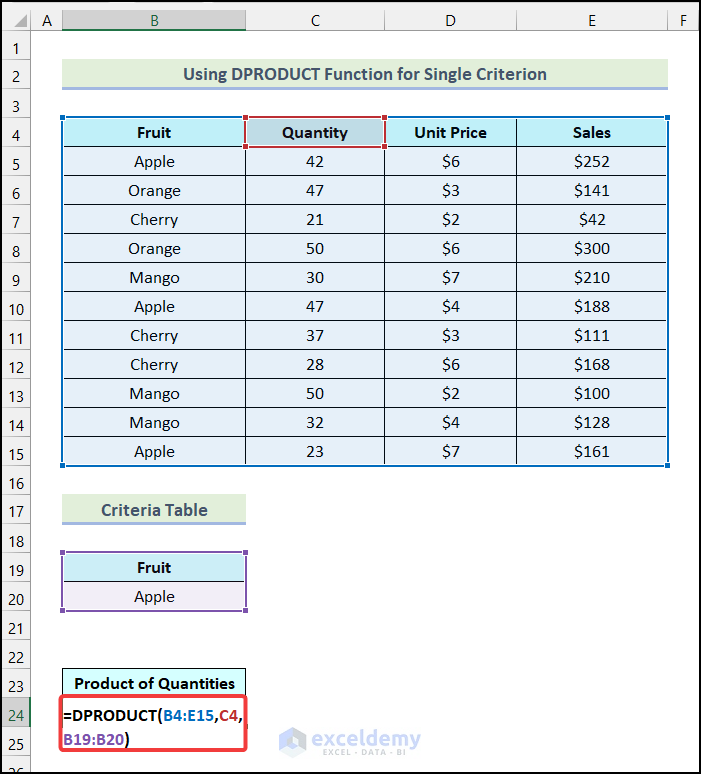
The sample dataset showcases Sales Data. To find the product of Quantities that match specific criteria:
Example 1 – Using the DPRODUCT Function with a Single Criterion
Steps:
- Create a Criteria Table and the output table.
The criterion is Apple (here).
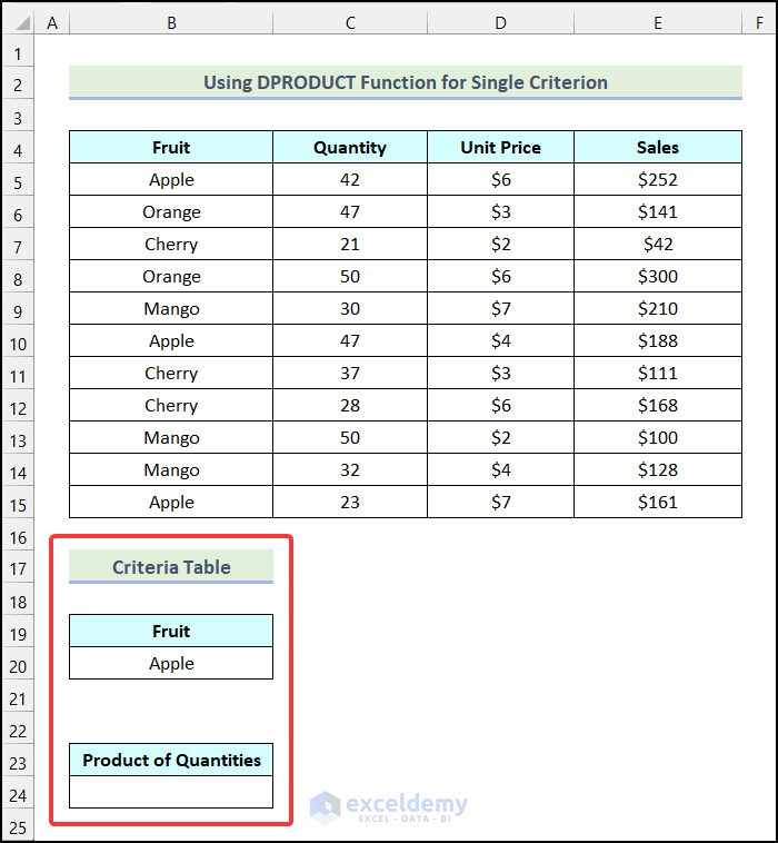
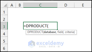
- Use the following formula in B24.
=DPRODUCT(B4:E15,C4,B19:B20)B4:E15 indicates the database, C4 is the heading of the Quantity column, and B19:B29 represents the criteria.
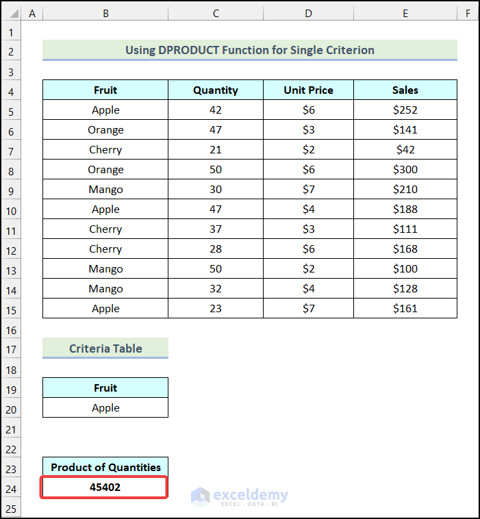
- Press ENTER.
This is the output.
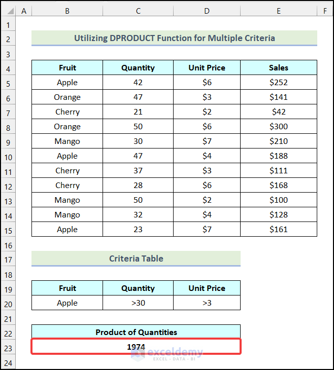
Example 2 – Utilizing the DPRODUCT Function with Multiple Criteria
Steps:
- Create a Criteria Table and the output table.
The three criteria are:
- Apple.
- Quantity greater than 30.
- Unit price more than $3.
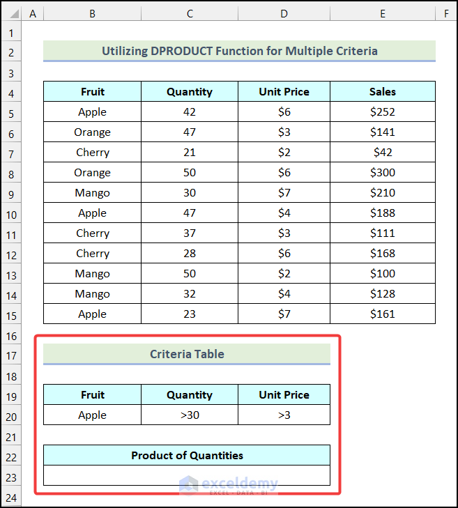
- Use the following formula in B23.
=DPRODUCT(B4:E15,C4,B19:D20)B19:D20 indicates the range in the Criteria Table.
- Press ENTER.
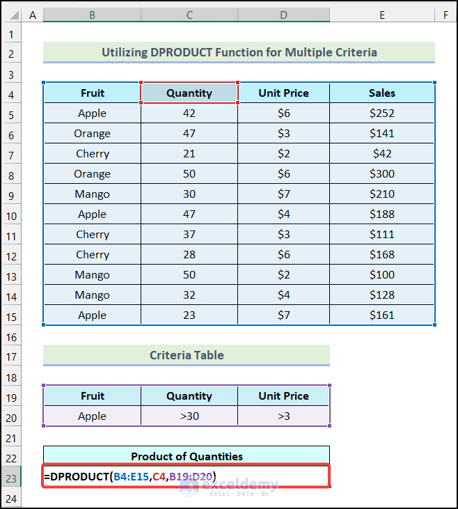
You will see the Product of Quantities that match the Criteria Table, in B23.
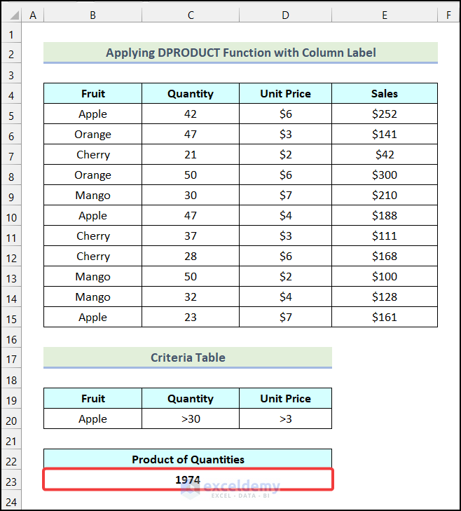
Example 3 – Applying DPRODUCT Function with Column Label in Field Argument
Steps:
- Use the following formula in B23.
=DPRODUCT(B4:E15,"Quantity",B19:D20)“Quantity” represents the field argument.
- Press ENTER.
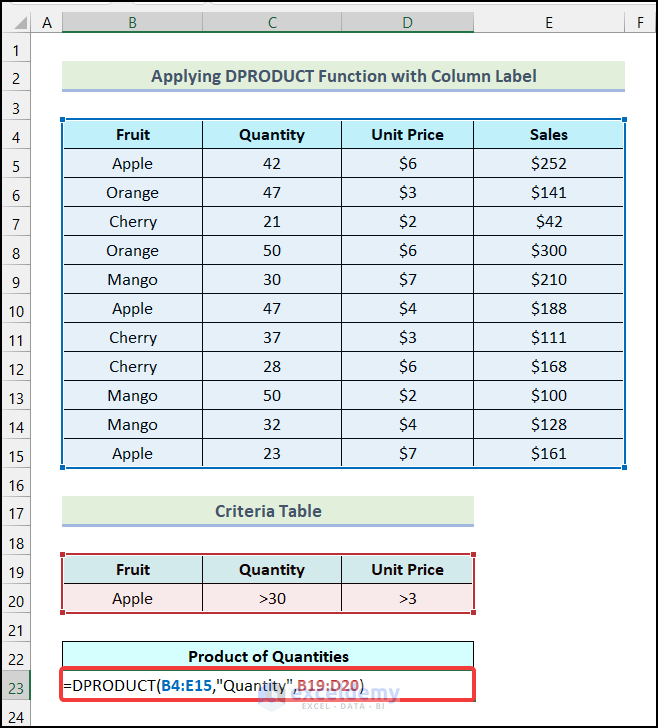
You will see the Product of Quantities in B23.
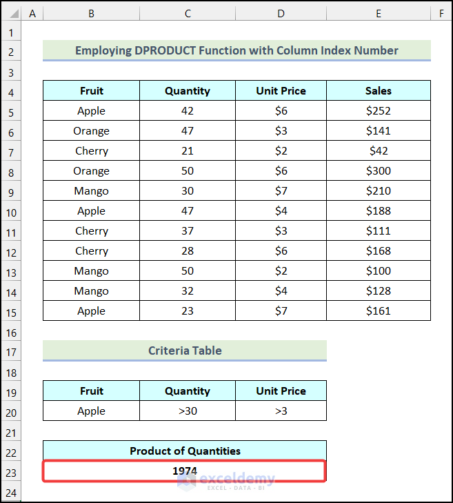
Example 4 -Using the DPRODUCT Function with the Column Index Number in the Field Argument
Steps:
- Use the following formula in B23.
=DPRODUCT(B4:E15,2,B19:D20)2 is the column index number: the field argument.
- Press ENTER.
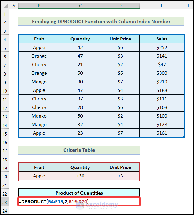
This is the output.
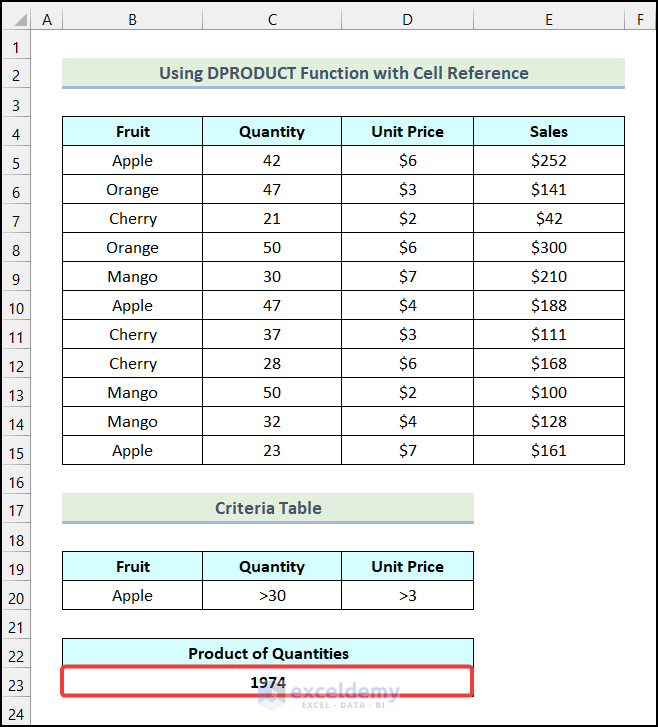
Example 5 – Using the DPRODUCT Function with a Cell Reference in the Field Argument
Steps:
- Use the following formula in B23.
=DPRODUCT(B4:E15,C4,B19:D20)C4 indicates the column header of the 2nd column: the field argument.
- Press ENTER.
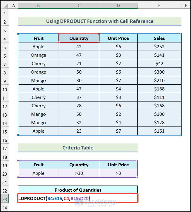
This is the output.
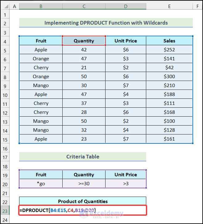
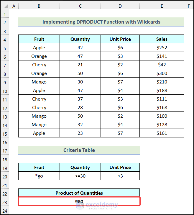
Example 6 – Using the DPRODUCT Function with Wildcards
Below are examples of wildcard criteria:
| Criteria with Wildcard | Meaning |
|---|---|
| Pen | Exactly matches “Pen”. |
| *en | Ends with “en”. |
| Pe* | Starts with “Pe”. |
Steps:
- Create a Criteria Table.
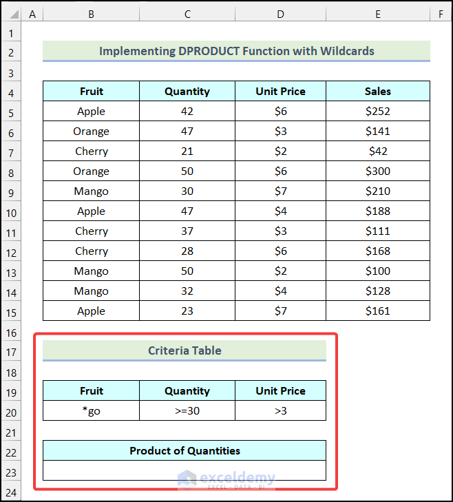
- Use the following formula in B23.
=DPRODUCT(B4:E15,C4,B19:D20)In the Criteria Table, “*go” refers to a word ending in “go“, and >=30 indicates the Quantity should be greater than or equal to 30.
- Press ENTER.
This is the output.
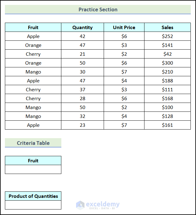
Practice Section
Practice here.
Download Practice Workbook
<< Go Back to Excel Functions | Learn Excel
Get FREE Advanced Excel Exercises with Solutions!
