Introduction to the Excel PMT Function
- Summary
The PMT function calculates the payment for a loan based on a constant interest rate. For instance, you have a 10- year home loan of $110,000 with an interest rate of 3%. Using the PMT function, you can calculate the periodic payment for the loan.
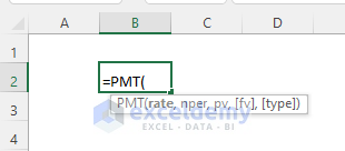
- Syntax
PMT(rate, nper, pv, [fv], [type])
- Arguments
| Argument | Requirement | Explanations |
|---|---|---|
| rate | Required | The interest rate of the loan. |
| nper | Required | The total number of payments. |
| pv | Required | The present value: the total value of all the loan payments at present (the original amount borrowed). |
| fv | Optional | The future value: the cash balance you have after the last payment. If this parameter is omitted, the future value is assumed to be zero (0). |
| type | Optional | It specifies when the payment is due. If this parameter is 0 or omitted, the payments are due at the end of each period. If it is 1, the payments are due at the beginning of each period. |
- Return Value
The PMT function returns the loan payments as a number.
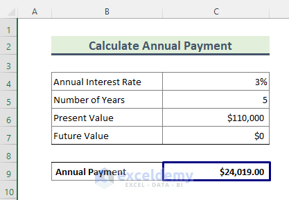
Example 1 – Calculate the Annual Payment Using the PMT Function
You have a 5-year home loan with an interest rate of 3%. The loan amount is $110,000. To calculate the annual loan payment:
Steps:
- Enter the following formula in C9.
=PMT(C4,C5,C6,C7)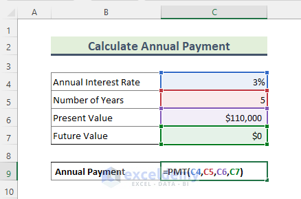
The [type] argument is not declared. By default, the payment will be due at the end of the period. If your loan payment is due at the beginning of the period, enter 1 as argument.
You will get the annual payment:
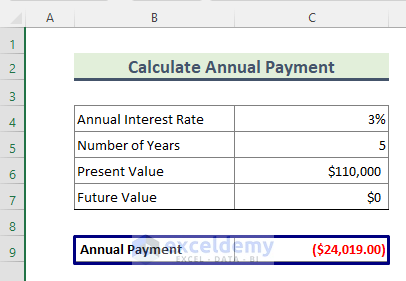
The result will be in currency format, red color, and rounded to two decimal places. By default, the result will be enclosed in parenthesis, which means the loan amount is negative.
Note:
To see the loan amount as a positive number, enter a minus (–) sign at the beginning of the PMT formula:
=-PMT(C4,C5,C6,C7)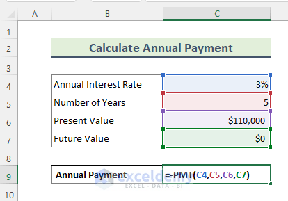
You will get a positive annual payment.
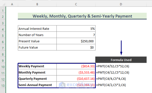
Example 2 – Applying the Excel PMT Function to Get Weekly, Monthly, Quarterly, and Semi-Annual Payments
You have to adjust the rate and nper arguments, depending on the number of payments per year:
- Divide the annual interest rate by the number of payments per year.
- For the nper, multiply the number of years by the number of payments per year.
Calculate loan payments for different periods for a 7-year home loan with an annual interest date of 5% and a loan amount of $250,000.
Steps:
- Enter the following formula in C10:C13.
The formula for the weekly payment is:
=PMT(C4/52,C5*52,C6)52 is used for the 52 weeks in a year.
The formula for the monthly payment is:
=PMT(C4/12,C5*12,C6)12 is used for the 12 months in a year.
=PMT(C4/4,C5*4,C6)For payments on a quarterly basis, calculate 4 times per year.
For a semi-annual payment, the formula is:
=PMT(C4/2,C5*2,C6)This is the output.
Example 3 – Use PMT Function to Determine the Periodic Loan Payment (In case of Down Payment)
You have bought a car for $30000 and as a down payment, you have paid 10% of the $30000. You have to pay the loan within 5 years at a 5% annual interest rate. Calculate the monthly payment:
Steps:
- Enter the following formula in C10.
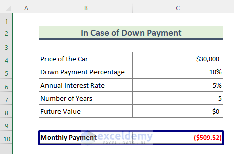
=PMT(C6/12,C7*12,C4*(1-C5),C8)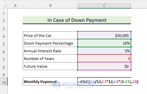
The price of the car is multiplied by (1-C5) which is C4*.9. You have to pay 90% of the price as a loan (as you paid 10% of the price as the down payment).
This is the output.
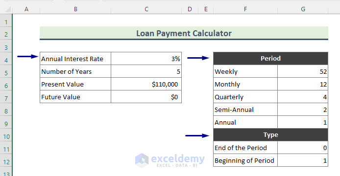
Example 4 – Create a Loan Payment Calculator Applying the PMT Function in Excel
Consider a 5-year loan amount of $110,000 with a 3% interest rate.
Steps:
- Enter the loan details in C4:C7 and prepare two lookup tables: Period (F5:G9) and Type (F11:G12).
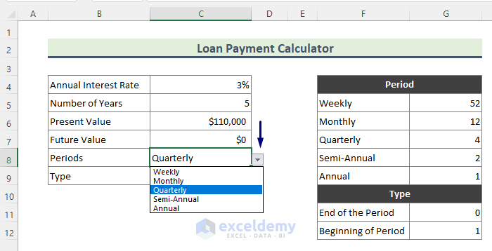
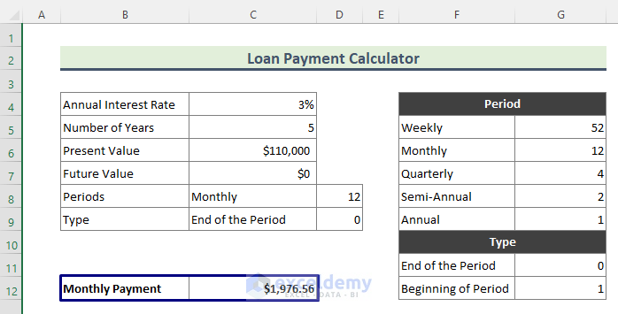
- Create a drop-down list for the periods (weekly, monthly, quarterly, semi-annual).
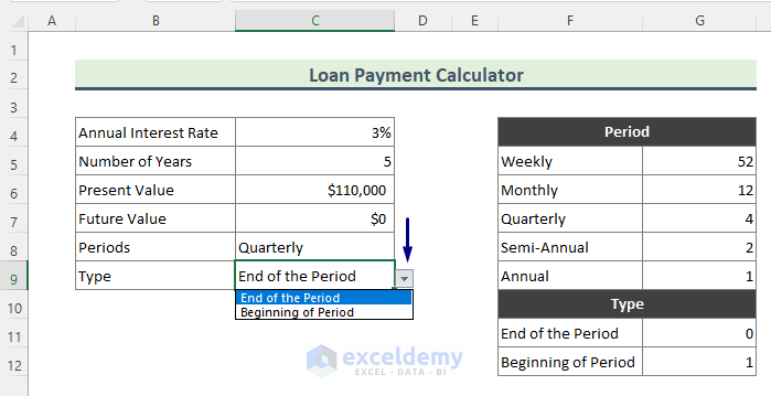
- Create a drop-down list for type (when payments are due).
- Use the combination of the IFERROR and VLOOKUP functions and enter the formula in D8.
=IFERROR(VLOOKUP(C8, F5:G9, 2, 0), "")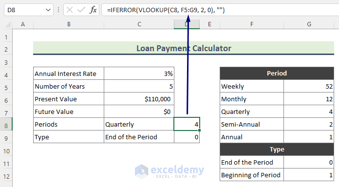
The VLOOKUP function finds the value of C8 in the lookup table Period and returns the periodic value according to the drop-down selection. The IFERROR function hides any error.
- Enter the following formula in D9.
=IFERROR(VLOOKUP(C9, F11:G12, 2, 0), "")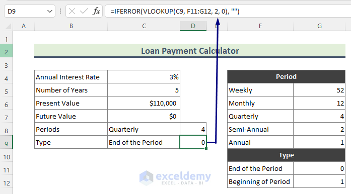
- To find the semi-annual payment, enter the formula in C12.
=IFERROR(-PMT(C4/D8,C5*D8,C6,0,D9),"")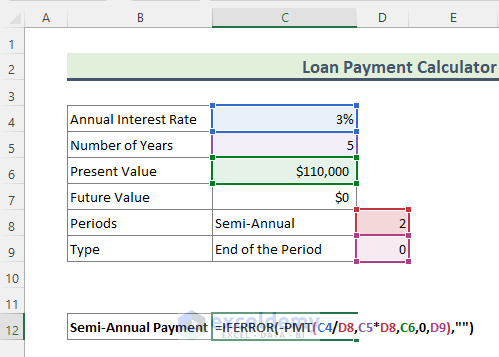
The PMT function calculates the loan payment. The IFERROR function hides errors.
You will see the semi-annual loan payment.
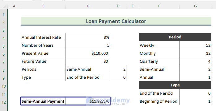
This is the output.
Things to Remember
- The payment returned by the PMT function includes only principal and interest rate. It does not include fees, taxes, or reserved amounts.
Common Errors of PMT Function
#NUM!: the rate argument is negative or the nper value is zero (0).
#VALUE!: one or more arguments are text values.
Download the Practice Workbook
Download the practice workbook.
<< Go Back to Excel Functions | Learn Excel
Get FREE Advanced Excel Exercises with Solutions!
