The methods below can be used even in large datasets to return any specific value that you need instead of an error.
Overview of Excel IFERROR Function
Description
The IFERROR function in Excel generates a custom value as a result if there is any error from the formula. If there is no error it will return the regular result.
Generic Syntax
=IFERROR(value, value_if_error)Argument Description
| ARGUMENT | REQUIREMENT | EXPLANATION |
|---|---|---|
| value | Required | The value, reference, or formula to check for an error. |
| value_if_error | Required | The set of independent data points. |
Returns
The specific value provided as the input for an error condition.
Available In
Excel for Office 365, Excel 2019, Excel 2016, Excel 2013, Excel 2011 for Mac, Excel 2010, Excel 2007, and Excel 2003.
How to Use IFERROR Function in Excel
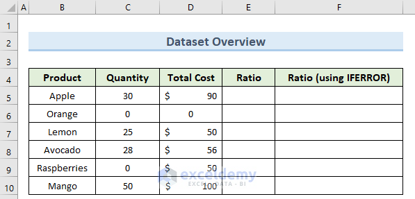
We’ll use a concise dataset to demonstrate, containing 5 columns – Product, Quantity, Total Cost, Ratio, and Ratio (derived using IFERROR). Initially, we keep all cells in General format besides the Total Cost column, which is in Accounting format.
Example 1 – Eliminating Basic Error
One of the most common uses of the IFERROR function in Excel is where there is the possibility of an error being returned.
Steps:
- In cell E5, insert the following formula:
=D5/C5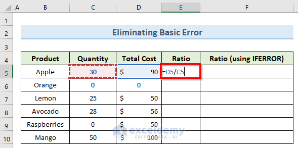
- Press Enter and copy this formula to the cells below using the Fill Handle.
Some #DIV/0! errors are returned, which we can eliminate using IFERROR.
- In cell F5, insert the following formula:
=IFERROR(E5,0)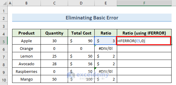
- Press Enter and copy this formula down to other cells using the Fill Handle.
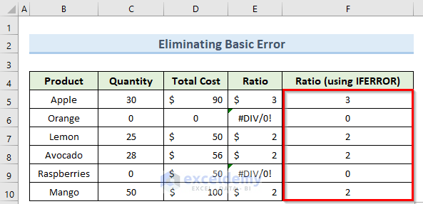
0 is now displayed instead of the errors.
Example 2 – Using IFERROR with an Array Formula
Steps:
- Double-click on cell F5 and enter the following formula:
=SUM(C5:C10/D5:D10)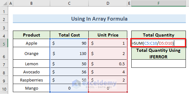
- Press Enter.
- Enter the following formula in cell F7:
=SUM(IFERROR(C5:C10/D5:D10,0))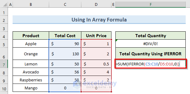
- Press Ctrl+Shift+Enter to apply the array formula.
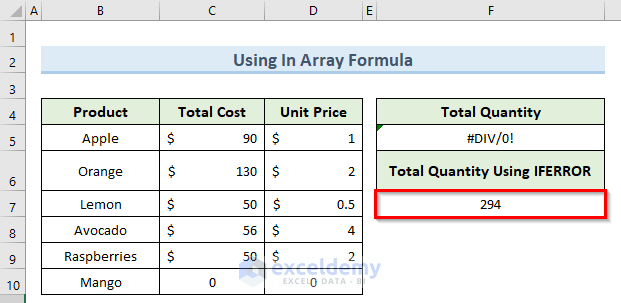
The error is removed.
Read More: How to SUM with IFERROR in Excel
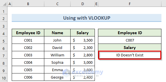
Example 3 – Applying IFERROR Function with VLOOKUP
It is very common to get an error if the value we are looking for doesn’t exist. You can combine the IFERROR function with the VLOOKUP function when looking up any value to resolve this.
Steps:
- Double-click on cell F7 and insert the formula below:
=IFERROR(VLOOKUP(F5,B4:D10,3,0),"ID Doesn't Exist")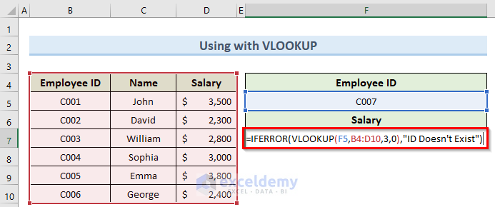
- Press Enter.
The message specified in the formula is now returned instead of an error value.
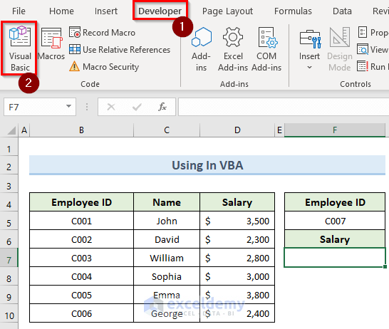
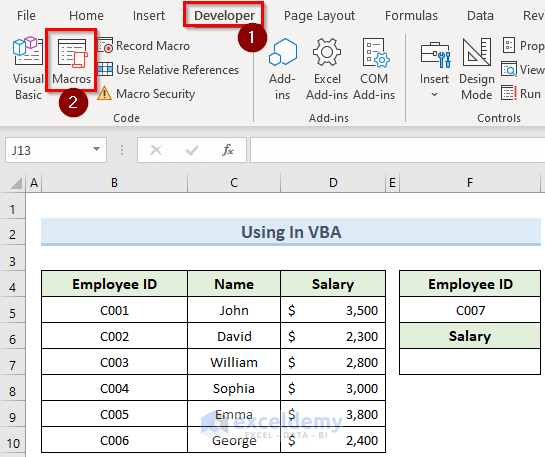
Example 4 – Using IFERROR Function In VBA
Steps:
- Click on the Developer tab and select Visual Basic.
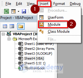
- Click Insert in the VBA window.
- Select Module from the list.
- Enter the formula below in the Module window that opens:
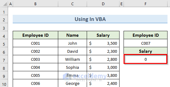
Sub IFERROR()
Range("F7").Formula = "=IFERROR(VLOOKUP(F5,B4:D10,3,0),0)"
End Sub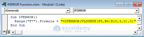
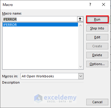
- Run the macro from the Developer tab by clicking on Macros.
- In the Macro window that opens, select the IFERROR macro and click Run.
As a result, the VBA code returns a value of 0 (which means the id is not present) instead of an error message.
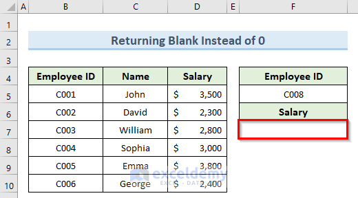
How to Use Excel IFERROR Function to Return Blank Instead of 0
In many cases, you might want to get a blank cell value instead of getting a 0 value whenever there is any sort of error.
Steps:
- In cell F7, enter the formula below:
=IFERROR(VLOOKUP(F5,B4:D10,3,0),"")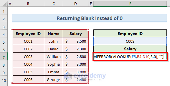
- Press Enter.
A blank cell value instead of an error message is returned.
Download Practice Workbook
Excel IFERROR Function: Knowledge Hub
- How to Use IF and IFERROR Combined in Excel
- How to Use Multiple IFERROR Statements in Excel
- How to Use Conditional Formatting with IFERROR in Excel
<< Go Back to Excel Functions | Learn Excel
Get FREE Advanced Excel Exercises with Solutions!
