If there is a cell with #N/A, #VALUE, or #REF! value in the selected range in which you want to apply the SUM function, it will return #N/A.
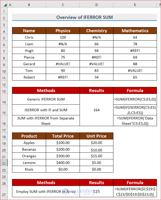
Method 1 – Generic IFERROR SUM in Excel
Steps:
- Select a cell to display the summation (F5).
- Enter the following formula and press ENTER.
=SUM(IFERROR(C5:E5,0))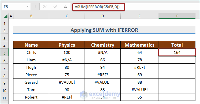
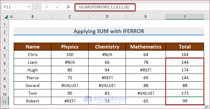
- Drag down the Fill Handle to see the result in the rest of the cells.
Formula Breakdown
Output: {100,0,64}
Output: 164
Read More: How to Use IFERROR with VLOOKUP in Excel
Method 2 – Using the SUM and the IFERROR in Array
Steps:
- Select a cell where you want to display the result (Here, D11).
- Enter the following formula to see the total quantity.
=SUM(IFERROR($C$5:$C$9/$D$5:$D$9,0))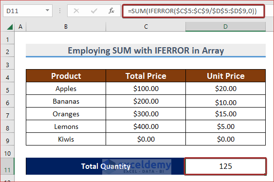
Formula Breakdown
Output: {5;20;20;80;0}
SUM({5;20;20;80;0}) —> returns the summation of those values.
Output: 125 (the “Total Quantity”)
- While working with arrays, remember to use the dollar sign ($) in front of the cell reference number.
- When working with array values, don’t forget to press Ctrl + Shift + Enter to extract results.
- After pressing Ctrl + Shift + Enter , you will notice that the formula is enclosed in curly braces {}, declaring it as an array formula. Don’t type the brackets {} , Excel does it automatically.
Read More: How to Use IF and IFERROR Combined in Excel
Method 4. Merging the ISERROR with the IF and the SUM Functions
Steps:
- Choose a cell (F5) and enter the following formula to see the SUM.
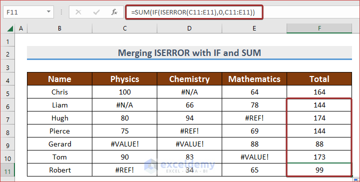
=SUM(IF(ISERROR(C5:E5),0,C5:E5))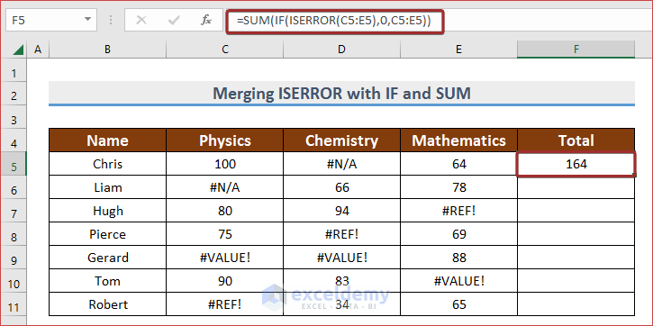
- Drag down the Fill Handle to see the result in the rest of the cells.
Formula Breakdown
Output: {FALSE,TRUE,FALSE}
IF({FALSE,TRUE,FALSE},0,C5:E5) —> returns 0 if the value is FALSE. Otherwise, it will return the value in C5:E5.
Output: {100,0,64}
SUM({100,0,64}) —> returns the summation.
Output: 164
Read More: Excel ISERROR vs IFERROR Functions
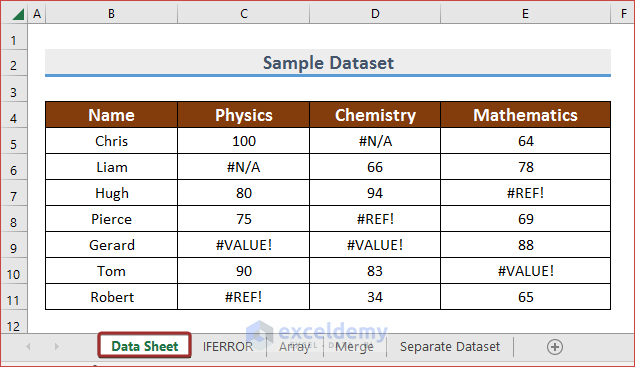
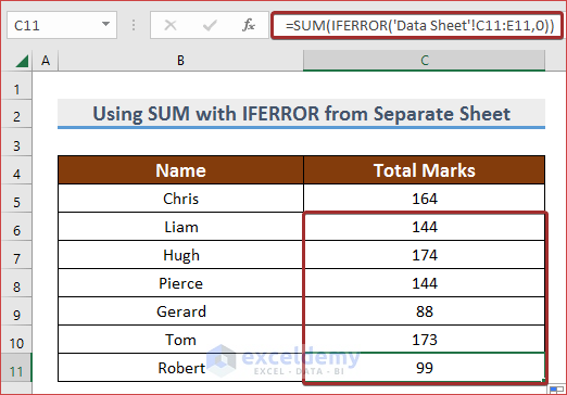
Method 4 – Use the SUM and the IFERROR in Separate Sheets
Save the previous dataset in a new sheet (“Data Sheet”).
In another worksheet (“Separate Dataset”), save space for the result value.
Steps:
- Select C5 and enter the following formula to get the sum considering #N/A, #VALUE, or #REF! as 0.
=SUM(IFERROR('Data Sheet'!C5:E5,0))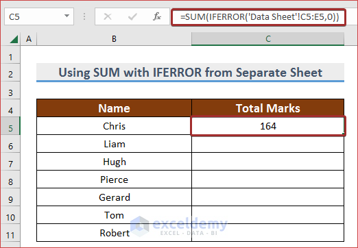
- Drag down the Fill Handle to see the result in the rest of the cells.
Download Practice Template
Download the free practice Excel template here and practice.
You May Also Like To Explore
- How to Use Conditional Formatting with IFERROR in Excel
- How to Use Multiple IFERROR Statements in Excel
- Excel IFERROR Function to Return Blank Instead of 0
<< Go Back to Excel IFERROR Function | Excel Functions | Learn Excel

