A DAX code will be used to find average sales, commission, success rate of broker calls, and the greatest number of calls.
Download Practice Workbook
Example 1 – Finding the Average Sales Using Power Pivot Measures
To create a pivot table:
- Select the whole dataset.
- Choose Insert >> Pivot Table >> From Table/ Range.
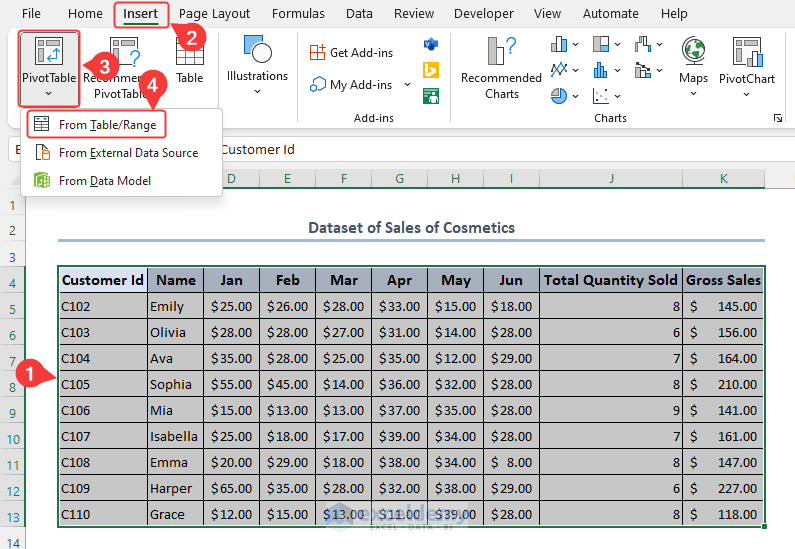
- Select a New Worksheet to create the PivotTable.
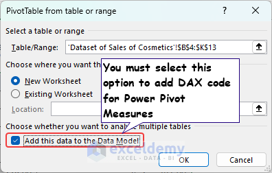
- Check Add this data to the Data Model and click OK.
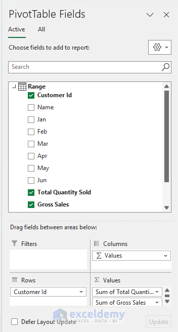
- Check the fields shown below.
- Right-click Range and select Add Measure.
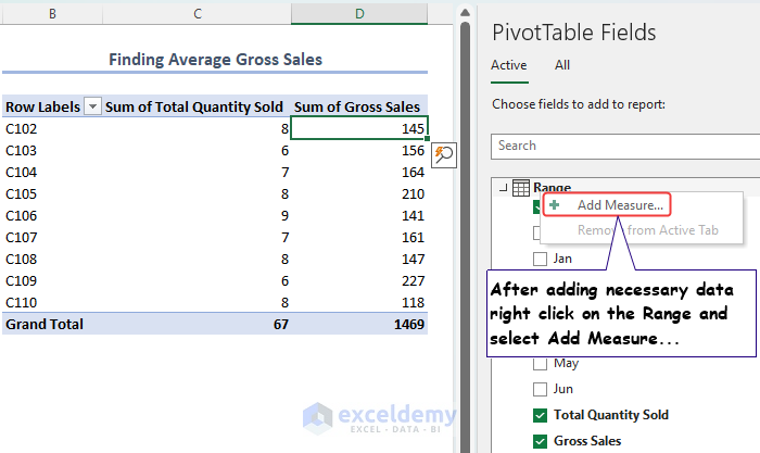
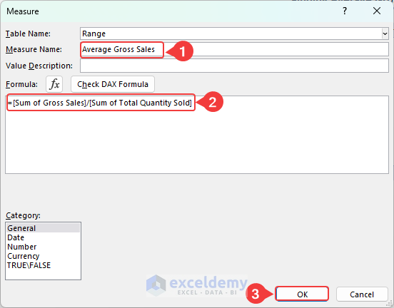
- Choose Average Gross Sales in Measure Name.
- Enter the following formula in the Formula box.
- Click OK.
=[Sum of Gross Sales]/[Sum of Total Quantity Sold]
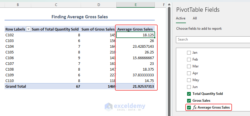
- Check Average Gross Sales to see the output.
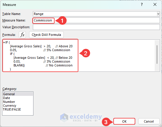
Example 2 – Finding the Commission Using Power Pivot Measure
- In the previous Pivot Table:
- Right-click Range in PivotTable Fields to create another Measure.
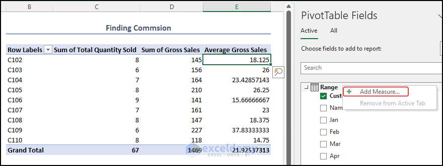
- Name the measure and enter the following DAX formula in the Formula box.
=IF (
[Average Gross Sales] > 20, // Above $20
0.05, // 5% Commission
IF (
[Average Gross Sales] < 20, // Below $20
0.03, // 3% Commission
BLANK() // No Commission
)
)
- Click OK.
Formula Breakdown The code snippet uses nested conditional statements to determine commission rates based on the value of Average Gross Sales. If the sales are above 20, a 5% commission rate is assigned; Below 20, a 3% rate is applied. Otherwise, no commission is given, returning a blank output.
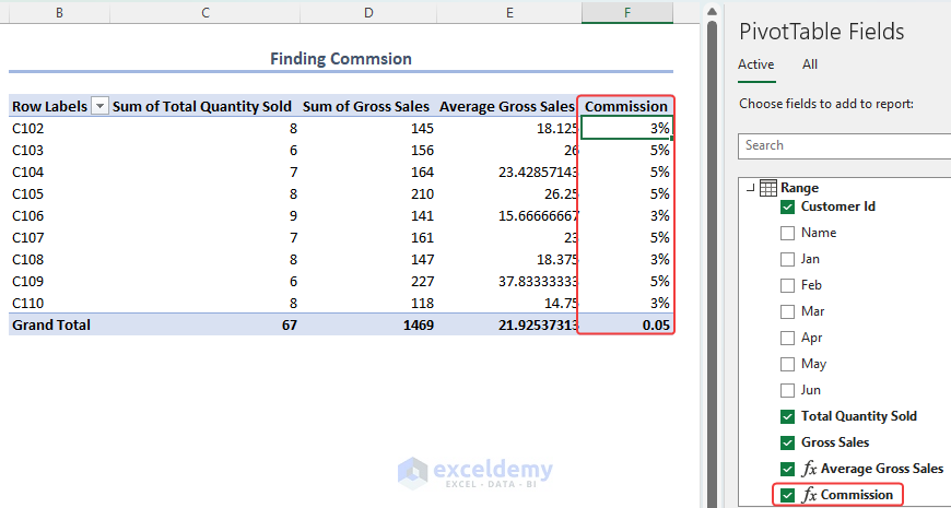
- Check Commission.
- This is the output. Use the Percentage.
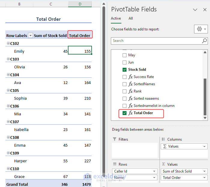
Example 3 – Finding the Total Order
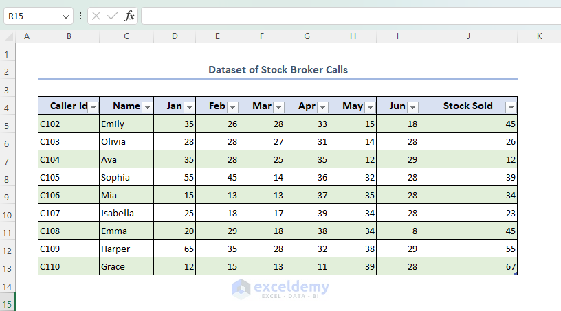
The dataset was modified and named Table3.
- Insert a pivot table.
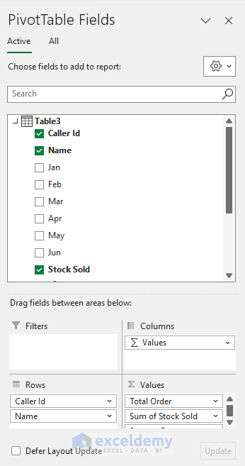
- Add a new Measure for Table3.
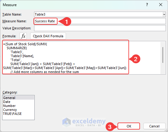
- Enter Total Order in Measure Name and use the DAX formula.
=SUMX(
SUMMARIZE(
'Table3',
'Table3'[Name],
"Total",
SUM('Table3'[Jan]) + SUM('Table3'[Feb]) + SUM('Table3'[Mar])+SUM('Table3'[Apr])+SUM('Table3'[May])+SUM('Table3'[Jun])
// Add more columns as needed for the sum
),
[Total]
)
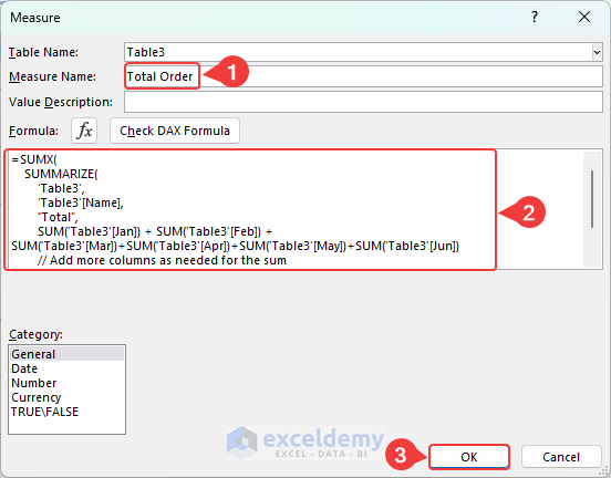
Formula Breakdown The DAX code uses the Power Pivot’s SUMMARIZE function to group data in Table3 by unique values in the Name column. Within each group, it calculates the sum of values for different months (Jan to Jun). The code creates a new calculated column called Total to store these sums. The outer SUMX function iterates through each group created by SUMMARIZE and calculates the sum of the Total column, resulting in the grand total of the calculated monthly sums for all names. This code computes the total value for each individual by summing their monthly data and provides an overall sum for all individuals combined.
This is the output.
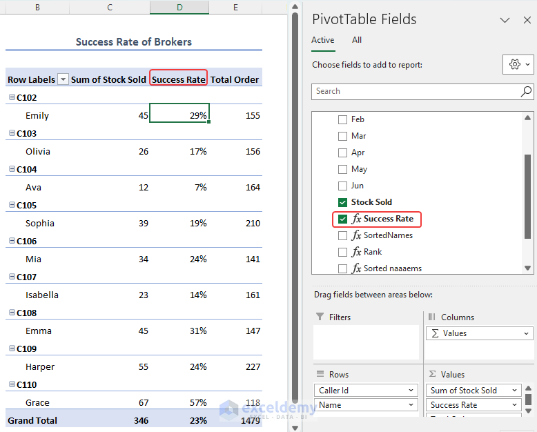
Example 4 – Finding the Success Rate
- Insert a pivot table.
- Add measures.
- Add Success Rate in Measure Name and enter the DAX formula.
=[Sum of Stock Sold]/SUMX(
SUMMARIZE(
'Table3',
'Table3'[Name],
"Total",
SUM('Table3'[Jan]) + SUM('Table3'[Feb]) + SUM('Table3'[Mar])+SUM('Table3'[Apr])+SUM('Table3'[May])+SUM('Table3'[Jun])
// Add more columns as needed for the sum
),
[Total]
)
Formula Breakdown The DAX formula calculates the ratio of Sum of Stock Sold to the total sum of monthly values (Jan to Jun) for each individual in the Table3. It groups data based on names, computing the sum of specified months for each group, and dividing the Sum of Stock Sold by the calculated total. The result offers insights into how the stock sold compares to an individual’s overall monthly activity, aiding in performance evaluation and analysis, and identifying the highest success rate.
This is the output.
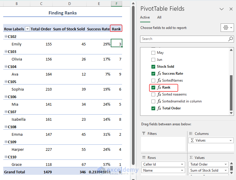
Example 5 – Ranking According to the Success Rate
- Insert a pivot table.
- Add measures.
- Add Rank in Measure Name and use the DAX formula.
=RANKX(ALL('Table3'), 'Table3'[Success Rate],, DESC)
![]()
Formula Breakdown The DAX formula calculates the rank of each individual in Table3 based on their Success Rate values. It considers all rows in Table3, orders them in descending order, and assigns a unique rank to each individual based on their relative performance.
This is the output.
Things to Remember
- Measures can be reused across multiple reports.
- Keep measures concise and relevant.
Frequently Asked Question
1. How do I troubleshoot when a measure displays unexpected results?
Double-check your DAX formula, filters, slicers, validate your source data and measure logic for accuracy.
2. Are Power Pivot measures compatible with Power BI?
Measures may need adjustments when transitioning between the two platforms.
3. How do I optimize performance when working with Power Pivot measures?
Limit complex calculations, avoid circular references, and optimize your data model for a better performance.
<< Go Back to Power Pivot Formulas | Power Pivot Excel | Learn Excel
Get FREE Advanced Excel Exercises with Solutions!
