Latest Posts From Joyanta Mitra

A DAX code will be used to find average sales, commission, success rate of broker calls, and the greatest number of calls. Download Practice ...

Method 1 - Making Correction to an Image Get picture format, you have to select the image first in every case. Choose Picture Format option from ...

Function 1 – TEXT Function Syntax: =TEXT(value, format_text) Arguments Explanation: Argument Required/Optional Explanation ...
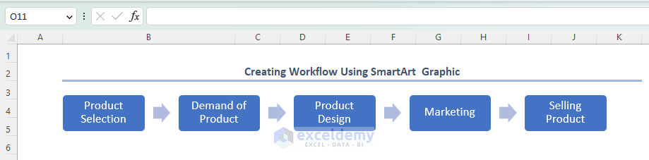
In this article, we provide a detailed guide to creating and automating workflow in Excel using Excel's built-in shapes. Creating a workflow can be a ...

This is an overview. Download Practice Workbook Comments in Excel.xlsx How to Insert/Add Comments in Excel 1. Insert Comment in ...

Excel Distribution Chart: Knowledge Hub How to Create a Distribution Chart in Excel How to Plot Normal Distribution in Excel Plot Normal ...

Here's a simple overview of putting a comma separator for numerical values in Excel. Download the Practice Workbook How to Add Comma in ...

In this article, we have used PROB, fractional method, NORM.DIST and NORMDIST function to find out Excel probability. Here's an overview of the function. ...
Here is an overview. Download Practice Workbook Dictionary in Excel.xlsm Example 1 - Creating a Data Dictionary in Excel Using an Excel ...

In this Excel tutorial, you will learn how to insert the delta symbol in Excel. This article describes 7 different methods of inserting the delta symbol, ...
n the picture below, we have demonstrated an example of inserting a timestamp in Excel. Download the Practice Workbook Timestamp in Excel.xlsm ...
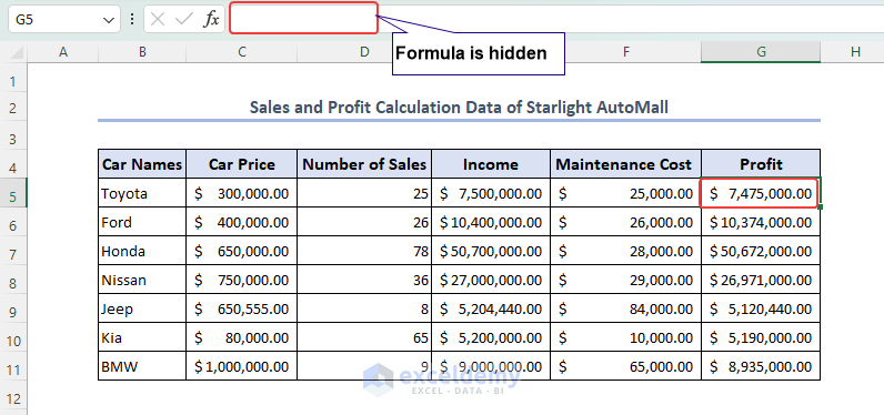
This article will cover how to hide Excel formulas, either by using the Format Cells and Review features, or with a VBA macro. Since these methods require ...
This is an overview. Method 1 - Using the RAND Function to Get a Random Decimal Number Between 0 and 1 Go to C5 and enter the ...

What Is Auto Formatting in Excel? Auto formatting in Excel simplifies the process of making your data visually appealing. It provides ready-made styles for ...

Numbering in Excel is essential for organizing, sorting, and referencing data, facilitating efficient data entry, and calculations, and enhancing clarity in ...
See Our Reviews at


Dear April
Thanks for your concern. There were some minor formatting issues with the VBA codes. Sorry for the inconvenience. We have updated our article. If you follow now, you will get the perfect calculator.
Thanks for your help
Regards,
Joyanta Mitra
ExcelDemy
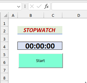
Dear Adam,

Thank you for your concern. You can not change the color of Excel button but you can use Command Button to change the button color.
You can follow the steps below to color your command button:
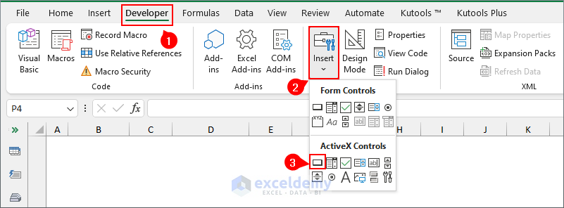
1. use Developer tab > Insert > ActiveX Controls > Command Button.
2. A command will appear and right click on it.
3. Choose CommandButton Object > Edit.
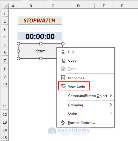
Name the button as Start.
4. Now right click on the command button and choose View Code.
5. Then write code below for starting.
Finally the button color has been added.
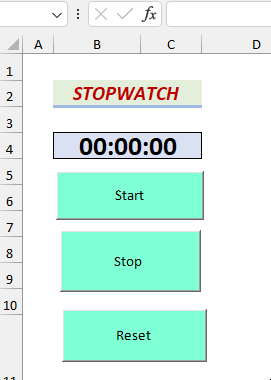
6. Now create a stop buttom and use the code below:
7. Write down the code for reset button:
Finally, you will have colored command button. You can change the color by changing color code 13959039.
Dear Kelley Sauer,
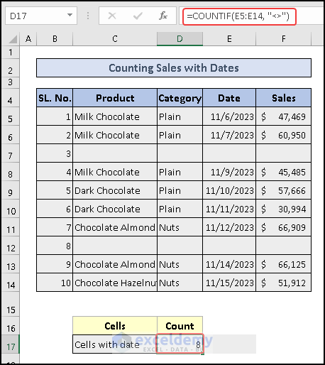
Please use this formula below to count sales having date.
=COUNTIF(E5:E14, "<>")It will count all sales with date. Using this formula, you will not get zero anymore. Moreover I have also used Ctrl+: to insert date.
With Regards,
Joyanta Mitra
Dear Anas,
You have to write the following code to get data validation for duplicate values, you have write the code below.
Then we get the data values of unique departments Marketing and Sales.
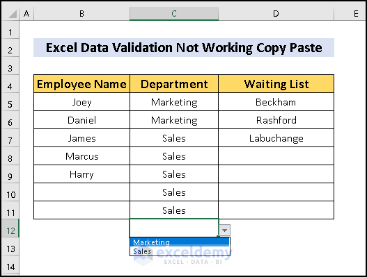
With regards,
Joyanta Mitra
Dear Santosh Kumar,
Please clarify the question. How can a person do more than 24 hours in 24 hours?
With Regards.
Joyanta Mitra
Dear FRANCESCA BATHE,
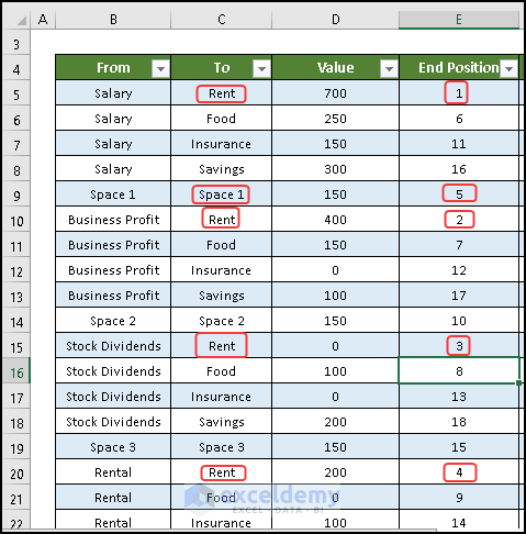
End Position is given according to column To. Where there is RENT in To column, the number starts 1,2,3,4 and ends with SPACE1 numbered 5. Then next is Food starting 6,7,8, 9 and ends with SPACE2 numbered 10. Likewise, numbering is done for every cell data in End Position.
Regards,
Joyanta Mitra
Code is alright. Please inform your particular problem.
Dear Prince,
Thank you very much for reading our article.
According to your query, 1st you wanted to know about a formula to create a drop-down list that will be used to select different types of leaves. You will get that in Step 3 of this article. In our Excel file, we selected leave using the drop-down list in Record sheet. Also when you move to any month leave information will be based on the Record sheet. So, information will not move from one month to another. Try this and hope you will get the solution.
Otherwise, send your Excel file with what you want to get and we will try to provide a solution. You can mail us at [email protected].
Thanks
Joyanta Mitra
ExcelDemy
Dear Karlyn Martinez,
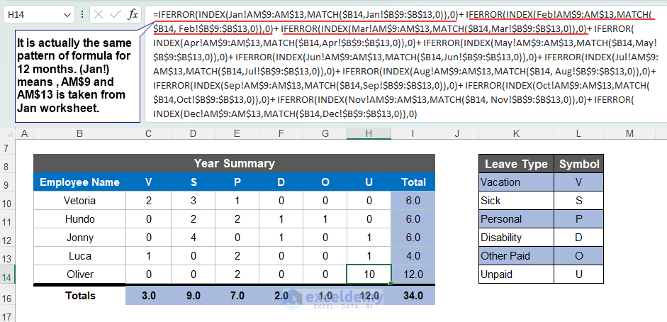
For your convenience, I have showed the task with following steps.
Steps:
● First, you have to recognize the pattern in the formula
● You can use Format Painter or drag the row to add a new row or rows for editing new data.
● Now add new data.
● Inset new rows in the Summary sheet.
● Insert the Entire row.
● Edit the code according to the main dataset. As now in Jan worksheet, new data is added, and so the range will be changed to AH$15 and $B$15.
Hope, this will be helpful for you.
Regards,
Joyanta Mitra
Excel & VBA Content Developer
This code will solve your problem. The code has a condition checking values blank or not.
Output:
Please write Ticker correctly both in your xlsx file and the code. Do not try to give invalid ticker or outdated ticker. Provide problems in detail for better service please.
First, you have to create different power queries for each worksheet for other tickers and copy the same code. Otherwise, it triggers the first. Then for 10 different tickers,the code is
this code creates 10 tables for 10 different tickers. You have to select one table according to Ticker and hover over the query in Workbook Query Section and press View in Worksheet. You will get the table have to create 10 sheets separately.