How to Use Conditional Formatting with the IFERROR Function in Excel – 4 Examples

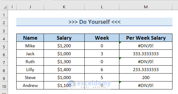
The dataset showcases Name, Salary, Week, and Per Week Salary.

To determine per week salary by dividing Salary by Week:

• Use the following formula in E5.

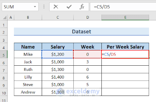
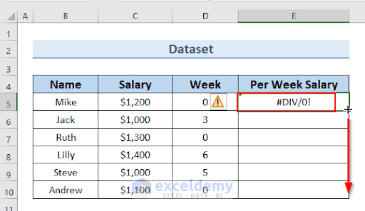
• Press ENTER.
• Since D5 contains 0, the result in E5 result is an error.
• Drag down the formula with the Fill Handle.

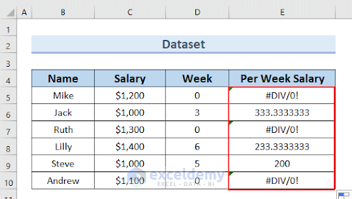
• There are several error values in this column.

You can  highlight these error values using Conditional Formatting.

Example 1 – Combining the IF and the IFERROR Functions to Highlight Errors

Combine the IF and IFERROR functions.

Steps:

• Select E5:E10.
• Go to the Home tab >> select Conditional Formatting >> select New Rule.

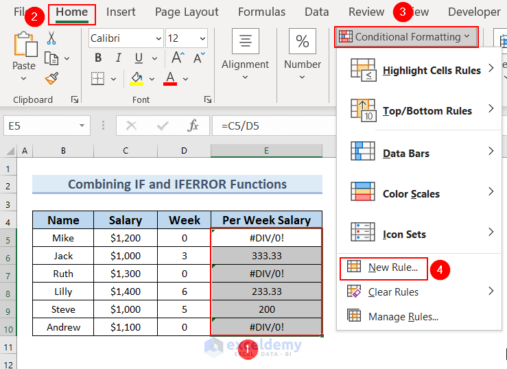
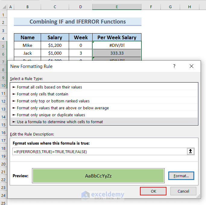
• In the New Formatting Rule dialog box, select Use a formula to determine which cells to format.
• Enter the following formula in Format values where this formula is true.

• Click Format.

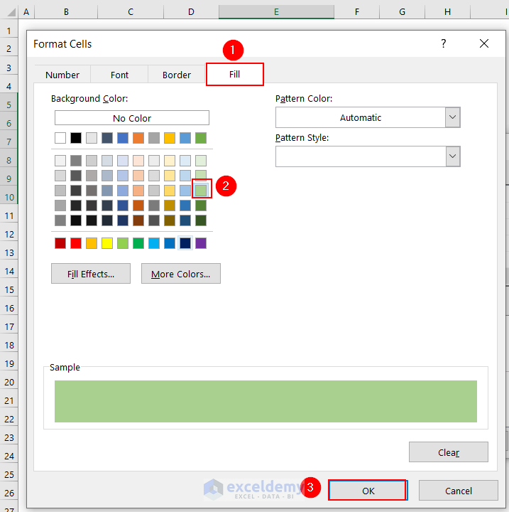
• In Fill  >> select a color. Here, light Green.
• You can see the Sample of the selected color.
• Click OK.

• Click OK in the New Formatting Rule dialog box.

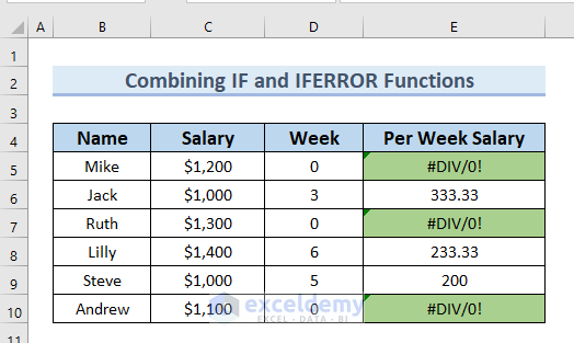
• Error values are highlighted in light Green.

Read More: How to Use IF and IFERROR Combined in Excel

Example 2 – Using the ISERROR Function

Use the ISERROR function.

Steps:

• Follow the steps described in Method 1 to display the New Formatting Rule dialog box.
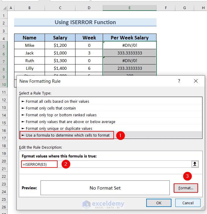
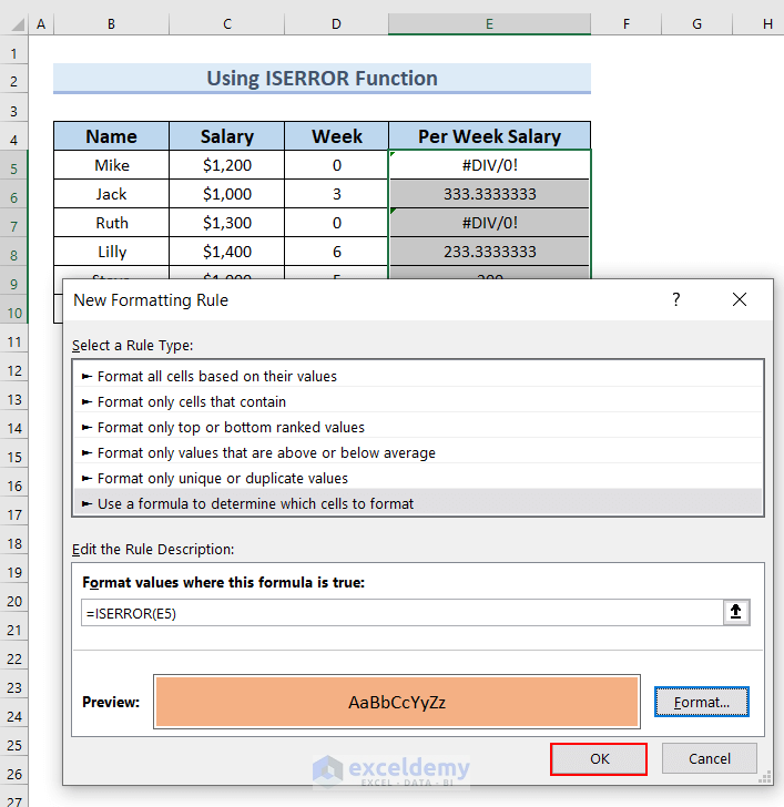
• Select Use a formula to determine which cells to format.
• Enter the following formula in Format values where this formula is true.

• Click Format.

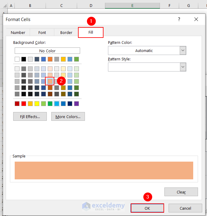
• In Fill  >> select a color. Here, light Pink.
• You can see the Sample of the selected color.
• Click OK.

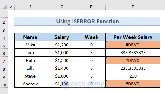
• Click OK in the New Formatting Rule dialog box.

• Error values are highlighted in light Pink color.

Example 3 – Formatting Cells With Errors Only

Steps:

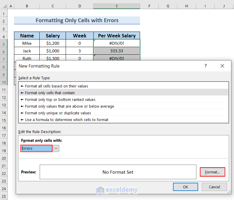
• Follow the steps described in Method 1 to display the New Formatting Rule dialog box.
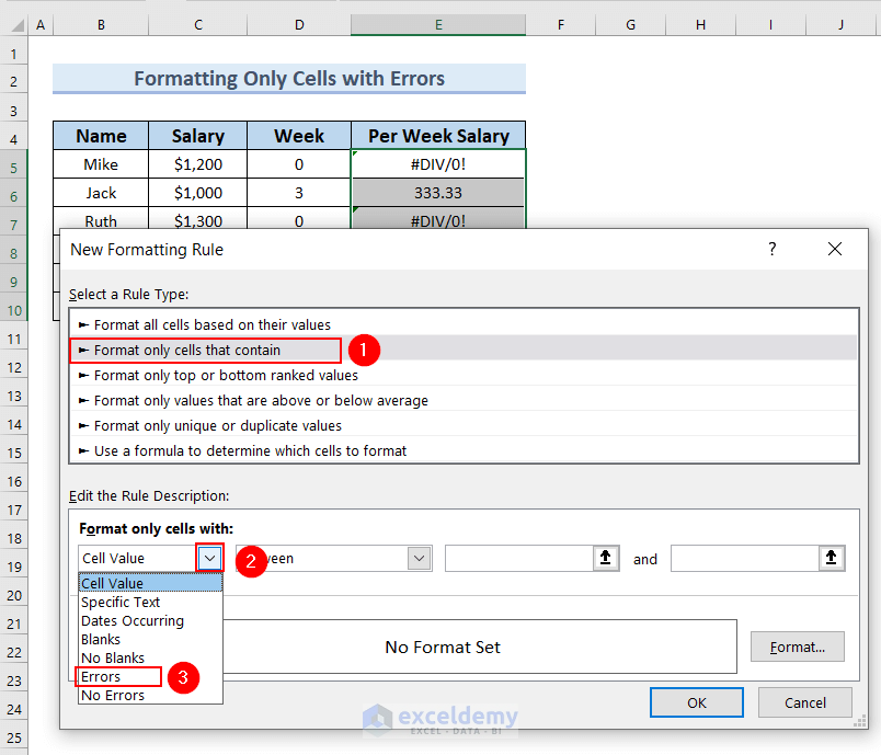
• Select Format only cells that contain.
• Click Format only cells with >> select Errors.

• Click Format.

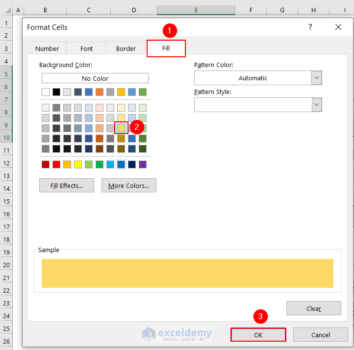
• In Fill group >> select a color. Here, light Yellow.
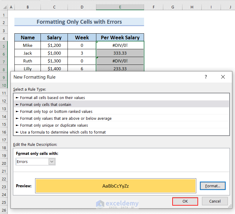
• You can see the Sample of the selected color.
• Click OK.

• Click OK in the New Formatting Rule dialog box.

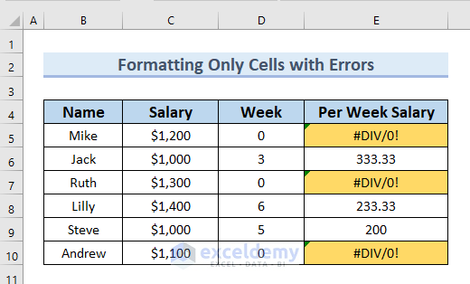
• Error values are highlighted in light Yellow.

Read More: How to Use IFERROR with VLOOKUP in Excel

Example 4 – Hiding Error Values by Applying Conditional Formatting

Convert errors to 0 using the IFERROR function, and hide the 0 values.

Steps:

• Enter the following formula in E5.

• The IFERROR function returns 0 when there is an error.

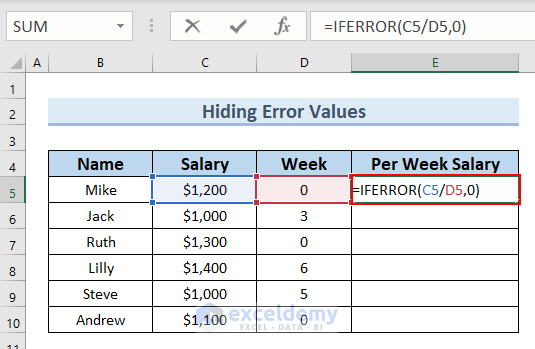
• Press ENTER.
• You can see the result in E5.
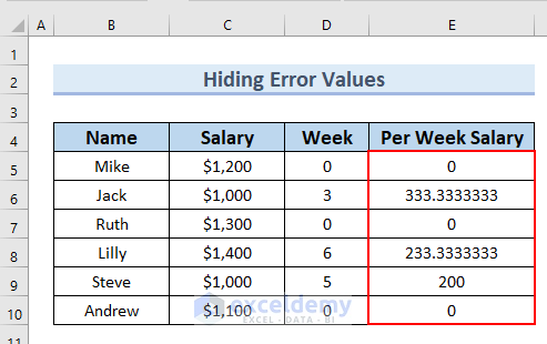
• Drag down the formula with the Fill Handle.

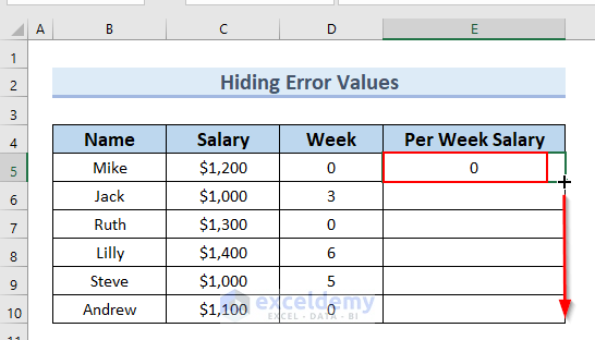
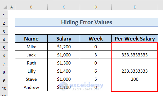
• In the Per Week Salary column, 0 replaced error values.
• Hide 0 values.

• Follow steps described in Method 1 to display the New Formatting Rule dialog box.
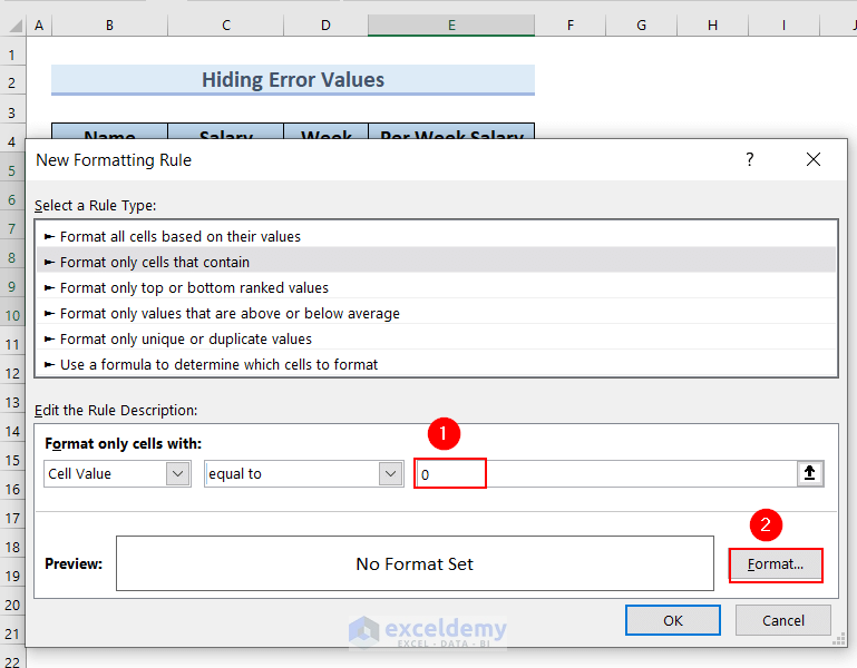
• Select Format only cells that contain.
• In Format only cells with: enter Cell Value in the first box.
• In the second box, select equal to.

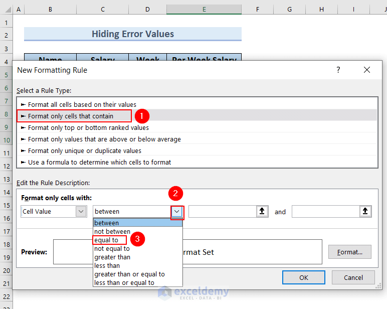
• In the third box, enter 0.
• Click Format.

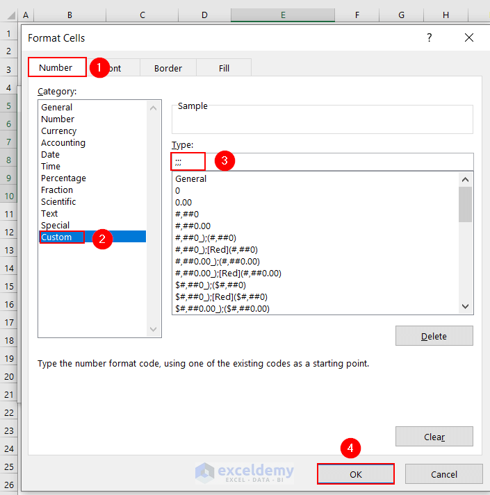
• In the Format Cells dialog box, in Number >> select Custom.
• Enter: ;;; (three semicolons) in Type.
• Click OK.

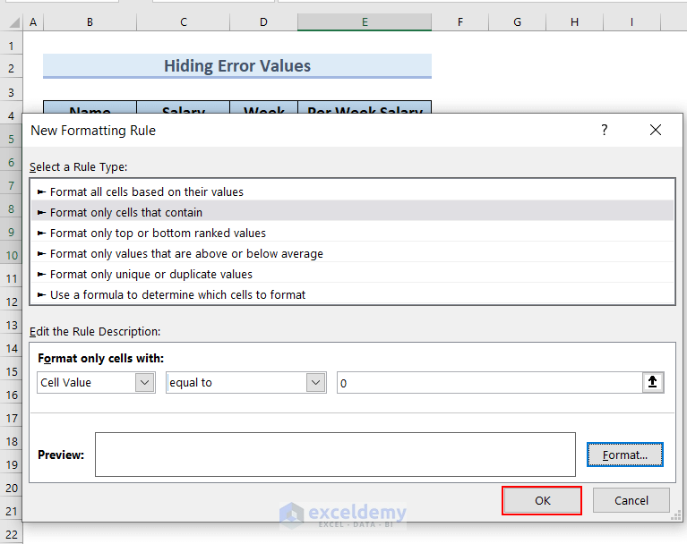
• Click OK in the New Formatting Rule dialog box.

• Error values are hidden.

Practice Section

Download the Excel file and practice.

Download Practice Workbook

Download the Excel file here.

Related Articles

• How to SUM with IFERROR in Excel
• How to Use Multiple IFERROR Statements in Excel
• Excel IFERROR Function to Return Blank Instead of 0

<< Go Back to Excel IFERROR Function | Excel Functions | Learn Excel