How to Use ISERROR Function in Excel (with 5 Examples)

If you are looking for how to use the ISERROR function in Excel then you are in the right place. For ignoring any type of calculation error, it is better to use exception handling. MS Excel provides an ISERROR function for this purpose. This function is categorized under Information functions. This article will share the complete idea of how the RIGHT function works in Excel independently and then with other Excel functions.

ISERROR Function in Excel (Quick View)

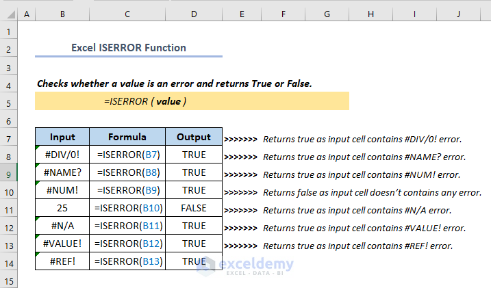
Excel ISERROR Function: Syntax & Arguments

Summary

This function indicates any error value (#N/A, #VALUE!, #REF!, #DIV/0!, #NUM!, #NAME?, or #NULL!).

Syntax

Arguments

Note: 

• In the argument, value is provided as a cell address, but we can use it to trap errors inside more complex formulas as well.
• This ISERROR function is available on Excel for Office 365, Excel 2019, Excel 2016, Excel 2013, Excel 2011 for Mac, Excel 2010, Excel 2007, Excel 2003, Excel XP, Excel 2000.

ISERROR Function in Excel: 5 Common Examples

Example 1: Finding Error Using ISERROR Function

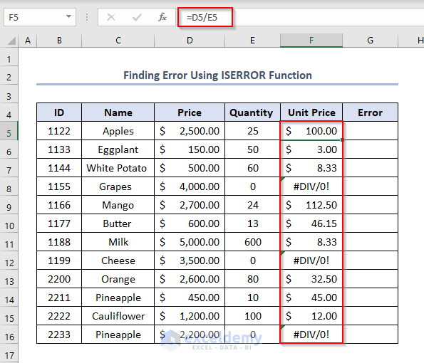
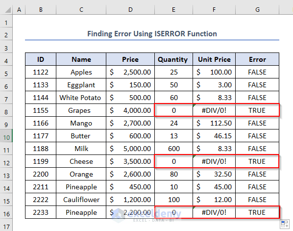
Let’s have a product dataset with their ID, Name, Total Price, and Quantity. Now we find Unit Price for each price we will divide the total price by quantity. Here some of the cells of the Quantity are missing or the value is 0 which will give #DIV/0! In Column F. Now the task is to find those error-contained cells using the ISERROR function.
We need to find if the error is False or True in Column G.

• Firstly, write the formula in the G5 cell like this.

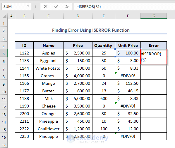
• Secondly, press ENTER.
• Thirdly, use the Fill Handle by dragging down the cursor while holding the right-bottom corner of the G5 cell like this.

• Consequently, we’ll get the output like this.
• Here, the #DIV/0! values in Column F will return TRUE as output in Column G and other normal values will return FALSE as output.

Example 2: Calculating Total Error Using SUMPRODUCT and ISERROR Functions

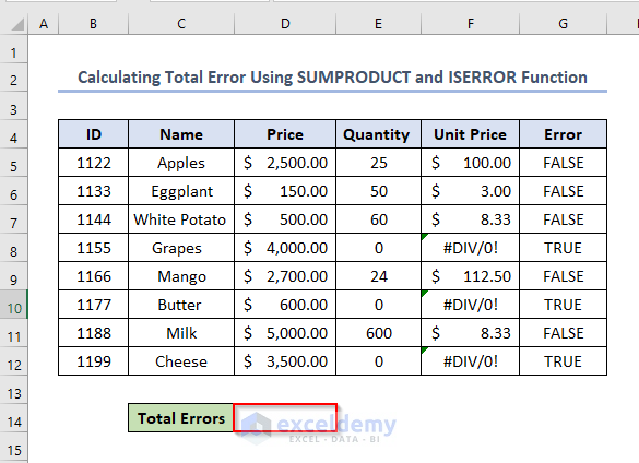
Now let’s count the total error that we have found in the first example. For this, we need to use the SUMPRODUCT function additionally.
Suppose, we want to find out the total number of errors of Column F in the D14 cell.

• Firstly, write the following formula in the D14 cell.

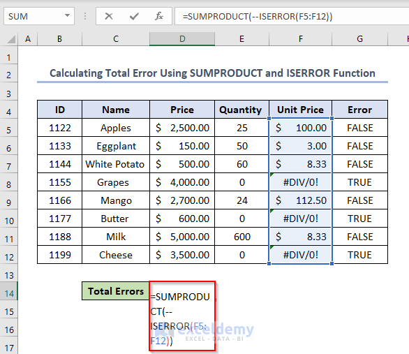
• Secondly, press ENTER to get the total number of errors as output. In this case, it is 3.

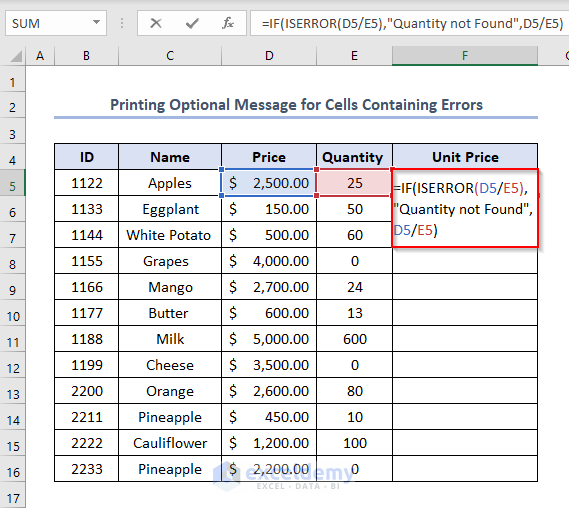
Example 3: Printing Optional Messages for Cells Containing Errors

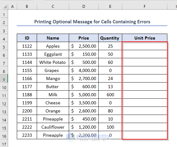
Instead of showing the error messages, we can show any message on the Unit Price cell using another additional function named the IF function. So, we will print a message “Quantity not Found” in Column F if the quantity is 0 instead of #DIV/0! Error.

• So, initially, write the formula in the F5 cell like this.

• Similarly, press ENTER.
• Thirdly, use the Fill Handle and we’ll get the output as Quantity Not Found where errors have occurred.

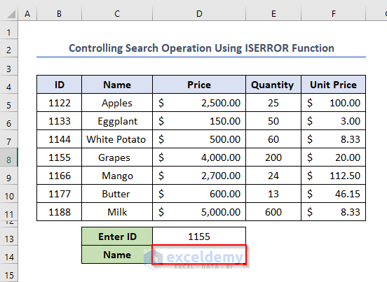
Example 4: Control Search Operation Using ISERROR Function

Now we will see how to search for anything and how to handle if there is a search item that is missing or not found in a particular dataset. We will search food names using their ID and show a message if the given input is not available on the dataset.
Suppose, we have an ID as 1155 in the D15 cell. We need to get the Food Name in the D16 cell.

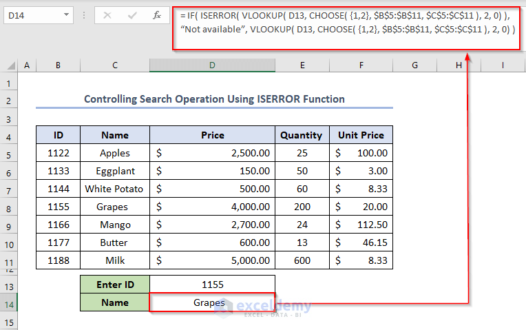
• Similarly, as before, write the formula in the D16 cell.

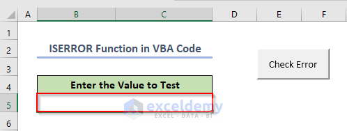
Example 5: ISERROR Function in VBA Code

Let’s see how we can detect any error contained in the cell using the button. There will be a code behind the button.

• Firstly, right-click on the Check Error > select Assign Macro.

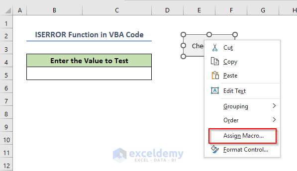
• Eventually, an Assign Macro window will appear.
• Secondly, click New.

• Eventually, a new module will appear.
• Thirdly, write the following code in the module.

Sub Button1_Click()

       'Display IsError function for cell B4 on Sheet6
        MsgBox IsError(Sheet6.Range("B4")), vb0k0nly, "Check Error"

Eng Sub

• Fourthly, click Run > select Run Sub/UserForm or click F5.

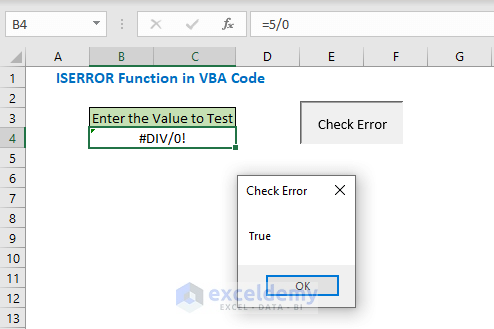
• Now type any number divided by 0 and click on the button to check the output.

IFERROR Vs ISERROR Functions in Excel

Both IFERROR and ISERROR functions find errors and give output but in a different way. The syntax of these two functions is also a little bit different.

The syntax of the IFERROR function is.

Eventually, the IFERROR function syntax has the following arguments.

• value The argument is checked for an error.
• value_if_error The value to return if the formula evaluates to an error. The following error types are evaluated:

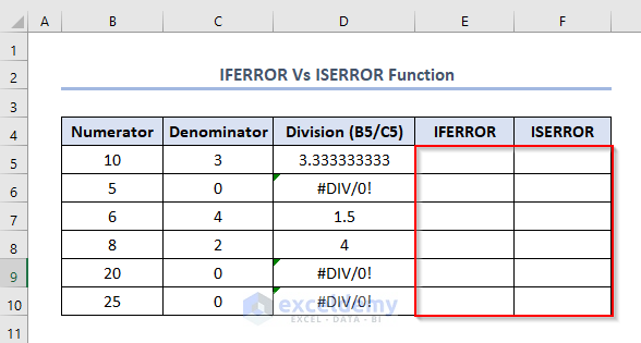
Suppose, we want to get errors as output in Columns E and F using IFERROR and ISERROR functions respectively.

• Firstly, write the formula in the E5 cell like this.

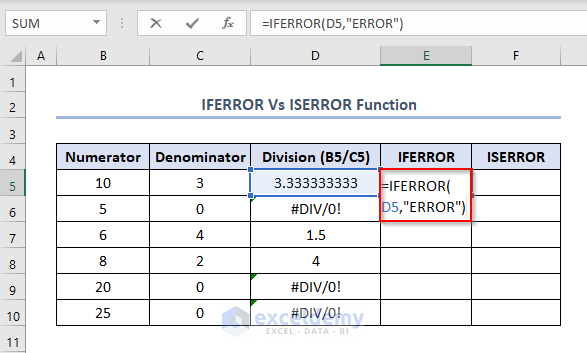
• If we press ENTER the error cells will give the output as ERROR.

On the other hand, the ISERROR function doesn’t give the output indicating ERROR directly.
It mainly gives the output showing TRUE or FALSE. By seeing this we can understand which cell has errors and which hasn’t.

• Similarly, as before, write the formula in the F5 cell like this.

• After pressing ENTER, we’ll get the output like this. Here the error cells will give output as TRUE.

Things to Remember

• This function tests for #N/A, #VALUE!, #REF!, #DIV/0!, #NUM!, #NAME?, and #NULL! Errors.
• It returns logical values, TRUE or FALSE.
• ISERROR function in Excel only checks if any given expression returns an error.

Download Practice Workbook

Conclusion

That’s all about the ISERROR function in Excel. Here I have tried to give a summary of this function and its different applications. Eventually, I have shown multiple methods with their respective examples but there can be many other iterations depending on numerous situations. If you have any inquiries or feedback, please let us know in the comment section.