VLOOKUP is a built-in Excel function. If you give a specific value in the VLOOKUP function it finds the value in a column and returns the corresponding value in another column. But, if the value is not found, it gives an error message (#N/A) which is sometimes not expected in a datasheet. This article mainly focuses on how you can omit the error message with the help of the ISERROR function and the VLOOKUP function in Excel. So, let’s get started.
How to Use ISERROR and VLOOKUP Functions in Excel: 3 Useful Ways
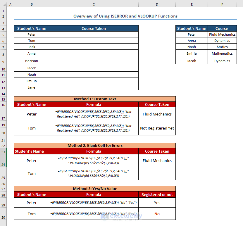
Sometimes, It is not very professional to show error messages in your datasheet. To create a polished workbook you must omit the error messages by applying different functions. Here, we have merged IF, ISERROR and VLOOKUP functions so that while using VLOOKUP function we can prevent having the error message. And most importantly we have shown how to replace the error with a custom text, blank cell, or Yes/No text which may work great in some real situations.
Method 1: Combining ISERROR, IF, and VLOOKUP Functions in Excel to Replace Errors with Custom Text
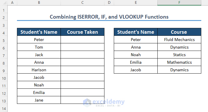
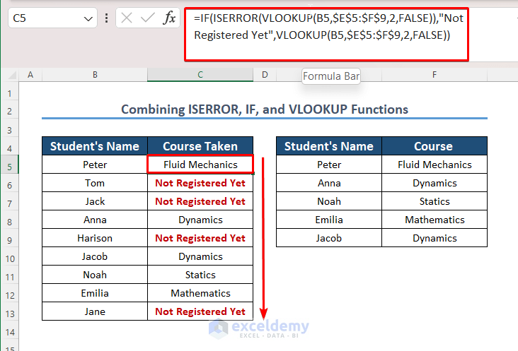
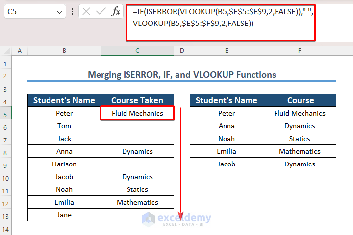
Suppose, We have a table that shows the name of the students and their corresponding Courses taken in a semester. We want to know each student’s corresponding course in another column without having any error message. Instead of an error message we want a custom text “Not Registered Yet”.
Following are the steps.
Steps:
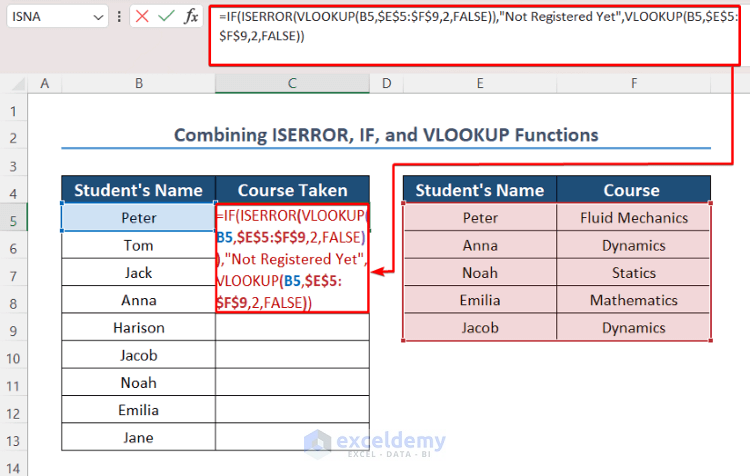
- Write the formula in cell C5.
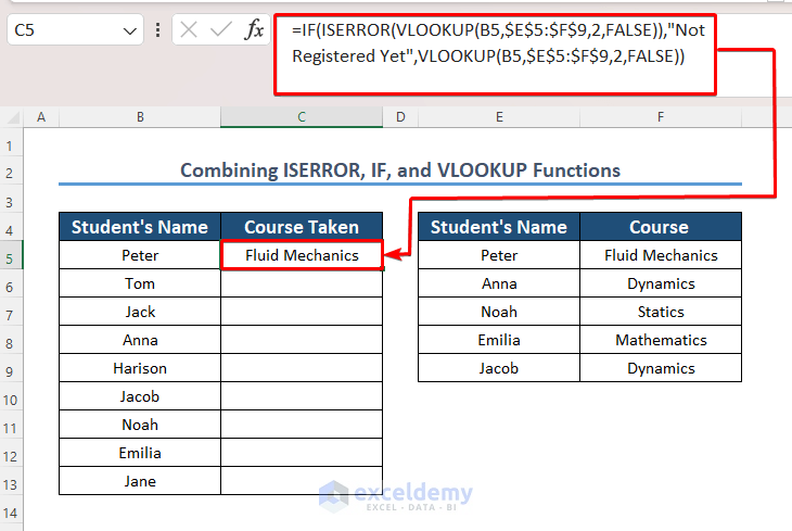
- To see the result, press ENTER.
- Therefore, we will get the Course Taken by Peter which is Fluid Mechanics.
- Lastly, we will copy the formula down to cell C13 by using the AutoFill feature.
- Consecutively, we can see that it returns our custom text where any student has not taken any course yet.
Formula Breakdown
- VLOOKUP(B5,$E$5:$F$9,2,FALSE), firstly, this portion looks up for (lookup value=B5) in (table array=E5:F9) and (column index=2). FALSE indicates the exact match of cell value B5.
- ISERROR(VLOOKUP(B5,$E$5:$F$9,2,FALSE)),”Not Registered Yet”,VLOOKUP(B5,$E$5:$F$9,2,FALSE), afterwards,the ISERROR function gives the (value=Not Registered Yet”) for error message.
- IF(ISERROR(VLOOKUP(B5,$E$5:$F$9,2,FALSE)),”Not Registered Yet”,VLOOKUP (B5,$E$5:$F$9,2,FALSE)), lastly, the IF function does the logical test, (value if true=”Not Registered Yet”) and (value if false =”lookup value”).
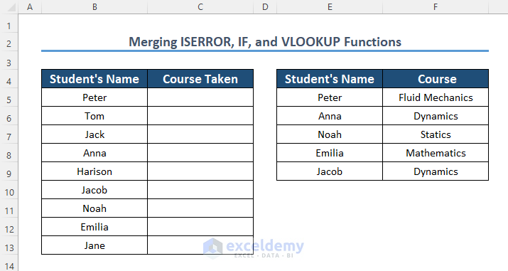
Method 2: Merging ISERROR, IF, and VLOOKUP Functions to Return Blank Cell for Errors in Excel
In case, you want to keep the error message cells blank, go after the steps below.
Steps:
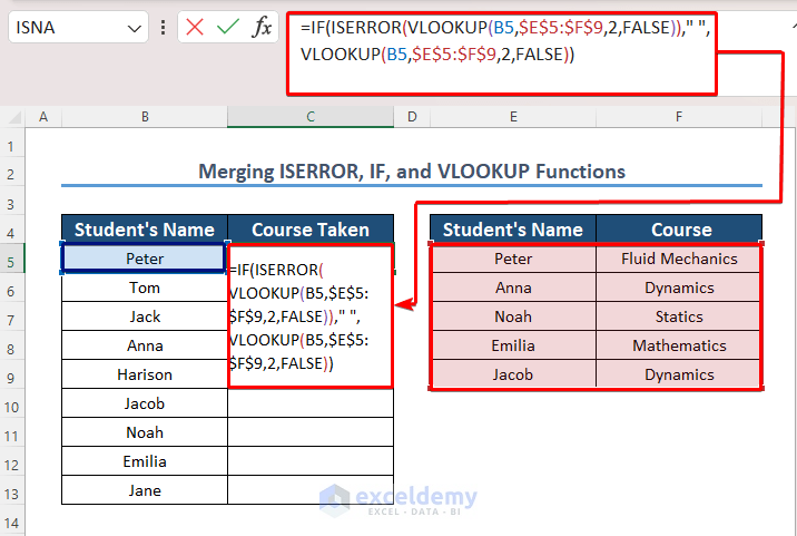
- Firstly, Put down the formula in cell C5.
- Then, click the ENTER.
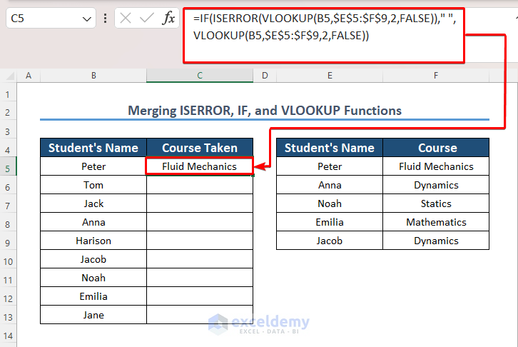
- Accordingly, we will get the output.
- Lastly, imitate the formula down through cell C13 by implementing the AutoFill feature.
- As a result, we will get the cells blank where error messages would appear.
Formula Breakdown
- VLOOKUP(B5,$E$5:$F$9,2,FALSE), in the first place, this portion looks up for (lookup value=B5) in (table array=E5:F9) and (column index=2). FALSE indicates the exact match of cell value B5.
- ISERROR(VLOOKUP(B5,$E$5:$F$9,2,FALSE)),” “,VLOOKUP(B5,$E$5:$F$9,2,FALSE), secondly, the ISERROR function delivered the (value=” “) which is a blank cell for #N/A.
- IF(ISERROR(VLOOKUP(B5,$E$5:$F$9,2,FALSE)),” “,VLOOKUP (B5,$E$5:$F$9,2,FALSE)), eventually, IF does the logical test, (value if true=” ”) and (value if false =”lookup value”).
Read More: IF with ISERROR Function in Excel
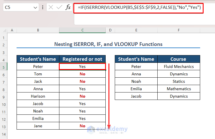
Method 3: Nesting ISERROR, IF, and VLOOKUP Functions to Get Yes/No Value
Wherever you need the output of the blank cells would show “No”, and the cells which carry value would show “Yes”, follow the instructions below.
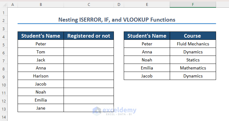
Steps:
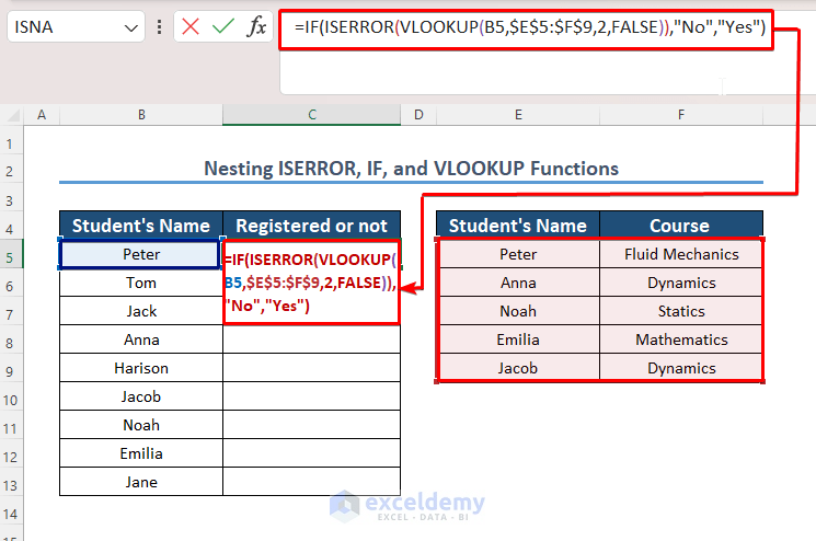
- In the first place, copy this formula in cell C5.
- Next, hit ENTER.
- As a result, we will get the value “Yes” as Peter has taken a course.
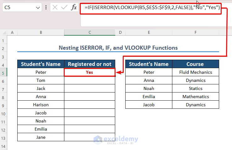
- Eventually, duplicate the formula down to cell C13. As a result, we got the Yes/No text in the cells.
Formula Breakdown
- VLOOKUP(B5,$E$5:$F$9,2,FALSE), So, this part of the formula looks up for (lookup value=B5) in (table array=E5:F9) and (column index=2).
- IF(ISERROR(VLOOKUP(B5,$E$5:$F$9,2,FALSE)),” “,VLOOKUP(B5,$E$5:$F$9,2,FALSE)), In conclusion, the IF function does the logical test (value if true=”No ”) and (value if false =”Yes”).
Read More: Nested IF and ISERROR Formula in Excel
Download Practice Workbook
You may download the following Excel workbook for better understanding and practice it by yourself.
Conclusion
This article shows 3 ways in which the IF, ISERROR, and VLOOKUP functions can be nested to get desired results. Hope this article will help to omit the error message while using the VLOOKUP function. Different situations may occur where these formulas need to be modified. If you face any problems regarding the formulas, please leave a comment. We will try to give the best possible solution.
<< Go Back to Excel ISERROR Function | Excel Functions | Learn Excel
Get FREE Advanced Excel Exercises with Solutions!
