IF with ISERROR Function in Excel: 4 Practical Examples

Here’s an overview of using the IF and ISERROR functions to check a car’s unit price depending on the amount of available stock.

What Is ISERROR in Excel?

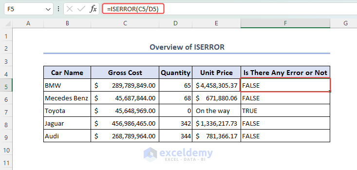
The ISERROR function in Excel is a logical function that allows users to check if a cell contains an error value. It returns a Boolean value TRUE if the cell contains an error, such as #VALUE!, #REF!, #DIV/0!, #N/A, #NUM!, or #NAME?. If the cell does not contain an error, the function returns FALSE.

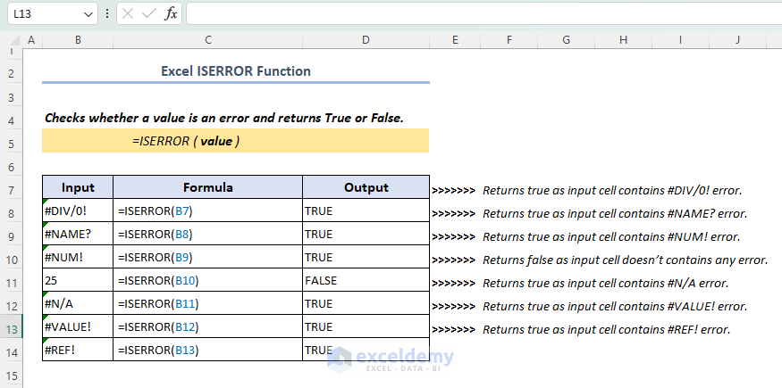
The ISERROR function is particularly useful when performing calculations or handling large datasets, as it helps identify and address potential formula errors.

IF with ISERROR Function in Excel: 4 Practical Examples

Example 1 – Combining IF with the ISERROR Function

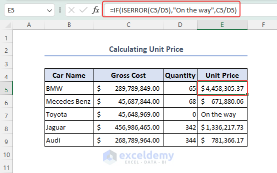
Case 1.1 – Determining the Unit Price of Cars

Consider the formula below in the E5 cell to find the unit price. When there are no units left in the Quantity column for the model, the cell will show the message “On the way”.

=IF(ISERROR(C5/D5),"On the way",C5/D5)

Formula Explanation

ISERROR(C5/D5): This part of the formula checks if the division of the value in cell C5 by the value in cell D5 results in an error. If there is an error, such as dividing by zero or encountering non-numeric values, the ISERROR function will return “TRUE”.
- Output: False
IF(ISERROR(C5/D5),”On the way”,C5/D5): The IF function evaluates the condition provided by ISERROR(C5/D5). If the condition is true (i.e., an error occurred during the division), the formula returns the text “On the way”. If the condition is false (i.e., no error occurred), the formula calculates the result of C5/D5.
- Output: $4,458,305.37

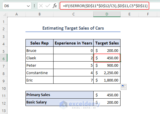
Case 1.2 – Estimating Target Sales of Cars

We used a formula in the D5 cell below to find the estimated sales of cars of a representative. As Bruce has no experience, he will get only Basic Salary.

=IF(ISERROR($D$11*$D$12/C5),$D$11,C5*$D$11)

C5 represents Experience in Years. $D$11 and $D$12 are Primary Sales and Basic Salary respectively. We use the dollar sign ($) in D11 and D12 cells to make those references absolute. These won’t be changed if we use the Fill Handle tool.

Formula Explanation

$D$11*$D$12/C5: This part of the formula calculates the result of multiplying the values in cells D11 and D12 and then dividing the product by the value in cell C5.
- Output: $450.
ISERROR($D$11*$D$12/C5): The ISERROR function checks if the calculation in step 3 results in an error. If there is an error (such as division by zero or encountering non-numeric values), it returns “TRUE“. Otherwise, it returns “FALSE“.
- Output: FALSE
IF(ISERROR($D$11*$D$12/C5),$D$11,C5*$D$11): The IF function evaluates the condition provided by ISERROR($D$11*$D$12/C5). If the condition is true (i.e., an error occurred during the calculation), the formula returns the value in cell D11. If the condition is false (i.e., no error occurred), the formula calculates the result of multiplying the value in cell C5 by the value in cell D11.
- Output: $450

Example 2 – Using a Combination of Excel IF, ISERROR, MATCH Functions

We have used the formula below in the C13 cell to find out whether a person has qualified for the job.

=IF(ISERROR(MATCH(B13, $C$5:$C$9, 0)), "No", "Yes" )

If name is found, then the output is “Yes”. Otherwise, it’s “No”.

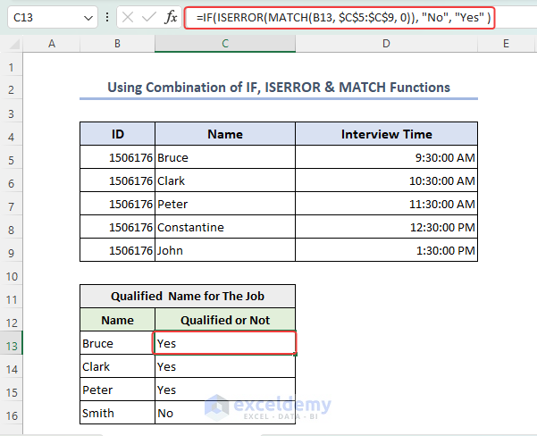
Formula Explanation

Step 1 – MATCH(B13, $C$5:$C$9, 0)

The searches for the value in cell B13 within the range $C$5:$C$9.
It looks for an exact match in the range.
If a match is found, it returns the relative position of the matching value within the range.
The last argument, 0, indicates that an exact match is required.
- Output: 1

Step 2 – ISERROR(MATCH(B13, $C$5:$C$9, 0))

The ISERROR function checks if the result of the MATCH function in Step 1 is an error.
If an error occurs (meaning the MATCH function couldn’t find a match for B13 in the range $C$5:$C$9), ISERROR will return TRUE.
If no error occurs (meaning the MATCH function found a match), ISERROR will return FALSE.
- Output: FALSE

Step 3 – IF(ISERROR(MATCH(B13, $C$5:$C$9, 0)), “No”, “Yes”)

The IF function evaluates the result of the ISERROR function in Step 2.
If the result is TRUE (indicating an error occurred), it returns the text “No”.
If the result is FALSE (meaning no error occurred), it returns the text “Yes”.
- Output: Yes

Example 3 – Using a Combination of IF, ISERROR, VLOOKUP Functions

We’ll extract the schedule of qualified members’ names from a primary dataset by using the formula below in C13:

=IF(ISERROR(VLOOKUP(B13,$C$5:$D$9,2,FALSE)),"Not Exist",VLOOKUP(B13,$C$5:$D$9,2,FALSE))

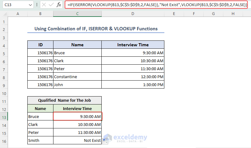
Formula Explanation

Step 1 – VLOOKUP(B13,$C$5:$D$9,2,FALSE)

The searches for the value in cell B13 (lookup_value) within the range $C$5:$D$9 (table_array).
It looks for an exact match in the leftmost column of the range.
If a match is found, it returns the corresponding value from the second column of the range ($C$5:$D$9) because the col_index_num is set to 2.
The range_lookup is set to FALSE, indicating an exact match is required.
- Output: 9:30:00 AM

Step 2 – ISERROR(VLOOKUP(B13,$C$5:$D$9,2,FALSE))

The ISERROR function checks if the result of the VLOOKUP function in Step 1 is an error.
If an error occurs (meaning the VLOOKUP function couldn’t find a match for B13 in the leftmost column of $C$5:$D$9), ISERROR will return TRUE.
If no error occurs (meaning the VLOOKUP function found a match), ISERROR will return FALSE.
- Output: False

Step 3 – IF(ISERROR(VLOOKUP(B13,$C$5:$D$9,2,FALSE)),”Not Exist”,VLOOKUP(B13,$C$5:$D$9,2,FALSE))

The IF function evaluates the result of the ISERROR function in Step 2.
If the result is TRUE (indicating an error occurred), it returns the text “Not Exist”.
If the result is FALSE (meaning no error occurred), it returns the result of the VLOOKUP function in Step 1.
- Output: 9:30:00 AM

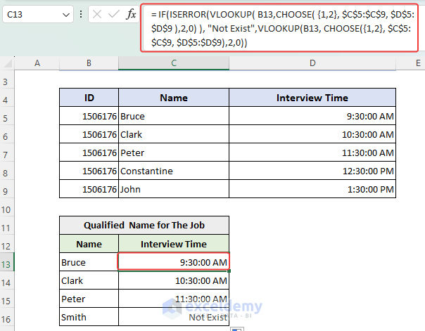
You can use the CHOOSE function with the VLOOKUP function to get the similar output. Instead of entering the table_array argument manually, we can apply the CHOOSE function to make an array. The formula is given below:

= IF( ISERROR( VLOOKUP( B13, CHOOSE( {1,2}, $C$5:$C$9, $D$5:$D$9 ), 2, 0) ), “Not present”, VLOOKUP( B13, CHOOSE( {1,2}, $C$5:$C$9, $D$5:$D$9 ), 2, 0) )

The formula CHOOSE({1,2}, $C$5:$C$9, $D$5:$D$9) in Excel is used to select a value from a list based on an index number. In this case, the index numbers are {1,2}, and the lists are located in cells C5:C9 and D5:D9.

The CHOOSE function will return an array of values corresponding to the selected index numbers. In this case, it will return the value from C5:C9 when the index is 1 and the value from D5:D9 when the index is 2. The value will be from D5:D9 which is 9:30:00 AM.

Example 4 – Applying IF and ISERROR Functions with an INDEX-MATCH Formula in Excel

We’ll track the names based on the interview times. We have used this formula in C13.

=IF(ISERROR(INDEX($C$5:$C$9, MATCH(B13, $D$5:$D$9, 0))), "Not qualified", INDEX($C$5:$C$9, MATCH(B13, $D$5:$D$9, 0)))

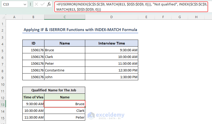
Formula Explanation

Step 1 – MATCH(B13, $D$5:$D$9, 0)

The MATCH function searches for the value in cell B13 within the range $D$5:$D$9.
It looks for an exact match in the range.
If a match is found, it returns the relative position of the matching value within the range.
The last argument, 0, indicates that an exact match is required.
- Output: 1

Step 2 – INDEX($C$5:$C$9, MATCH(B13, $D$5:$D$9, 0))

The INDEX function retrieves the value from the range $C$5:$C$9.
It uses the result of the MATCH function in Step 1 to determine the relative position of the value to retrieve.
The INDEX function returns the value from the corresponding position in the range $C$5:$C$9.
- Output: 9:30:00 AM

Step 3 – ISERROR(INDEX($C$5:$C$9, MATCH(B13, $D$5:$D$9, 0)))

The ISERROR function checks if the result of the INDEX function in Step 2 is an error.
If an error occurs (meaning the MATCH function couldn’t find a match for B13 in the range $D$5:$D$9), ISERROR will return TRUE.
If no error occurs (meaning the MATCH function found a match), ISERROR will return FALSE.
- Output:

Step 4 – IF(ISERROR(INDEX($C$5:$C$9, MATCH(B13, $D$5:$D$9, 0))), “Not qualified”, INDEX($C$5:$C$9, MATCH(B13, $D$5:$D$9, 0)))

The IF function evaluates the result of the ISERROR function in Step 3.
If the result is TRUE (indicating an error occurred), it returns the text “Not qualified”.
If the result is FALSE (meaning no error occurred), it returns the result of the INDEX function in Step 2.
- Output: 9:30:00 AM

Things to Remember

After using a formula, you may need to change the data type of the input or output cells.
While using the VLOOKUP function, be careful when selecting the table_array and inputting the col_index_num argument.

Frequently Asked Questions

How can I display a custom message when an error is detected using the nested IF and ISERROR functions?

To display a custom message when an error is detected, you can include a text value or message as the action_if_error parameter within the nested IF and ISERROR functions. For example, you can use =IF(ISERROR(A1), “Error: Invalid value”, A1) to display the custom message “Error: Invalid value” when cell A1 contains an error.

Can I use the nested IF and ISERROR functions to handle multiple error conditions?

Yes, you can use the nested IF and ISERROR functions to handle multiple error conditions by nesting multiple IF and ISERROR functions or combining them with other logical functions. By checking for different error types within separate nested IF and ISERROR functions or using logical operators like OR, AND, you can create complex conditions to handle various error scenarios.

Download the Practice Workbook

IF ISERROR.xlsx

<< Go Back to Excel ISERROR Function | Excel Functions | Learn Excel

Get FREE Advanced Excel Exercises with Solutions!

IF with ISERROR Function in Excel: 4 Practical Examples

What Is ISERROR in Excel?

IF with ISERROR Function in Excel: 4 Practical Examples

Example 1 – Combining IF with the ISERROR Function

Case 1.1 – Determining the Unit Price of Cars

Case 1.2 – Estimating Target Sales of Cars

Example 2 – Using a Combination of Excel IF, ISERROR, MATCH Functions

Example 3 – Using a Combination of IF, ISERROR, VLOOKUP Functions

Example 4 – Applying IF and ISERROR Functions with an INDEX-MATCH Formula in Excel

Things to Remember

Frequently Asked Questions

Leave a reply Cancel reply