Mahfuza Anika Era, Author at ExcelDemy

User Posts: Mahfuza Anika Era

How to Use Advanced Pivot Table in Excel (25 Tips & Techniques)

In this article, I have illustrated 25 powerful techniques and features of PivotTable. I have mostly covered advanced levels of Pivot Table in Excel. If you ...

Mahfuza Anika Era Sep 4, 2023

READ MORE +

Excel VBA to Comment Multiple Lines (3 Quick Steps)

If you want to comment on multiple lines in a VBA code to make the code easily understandable, this article can help you to do this in 3 simple steps. ...

Mahfuza Anika Era May 18, 2023

READ MORE +

How to Use Excel UserForm as Date Picker (with Easy Steps)

Date Picker is a type of calendar from which you can navigate through the months and years and insert the date into the cell. In an Excel UserForm, a date ...

Mahfuza Anika Era May 16, 2023

READ MORE +

Excel VBA to Activate Workbook with Partial Name

Remembering long Workbook names takes extra time and effort. Using VBA, you can activate a Workbook without remembering it’s full name. Isn’t it great? With ...

Mahfuza Anika Era May 14, 2023

READ MORE +

Excel VBA to Exit Select Case (with Examples)

Are you trying to exit a Select Case Statement for a specific condition in Excel VBA? It greatly helps to optimize the performance of the code. Unfortunately, ...

Mahfuza Anika Era May 11, 2023

READ MORE +

How to Move Excel Chart X Axis to Bottom (2 Simple Methods)

Are you trying to move the X-axis of your Excel chart to the bottom? There are so many cases where you need to place the X-axis or horizontal axis at the ...

Mahfuza Anika Era Oct 3, 2023

READ MORE +

How to Use DSTDEVP Function in Excel (2 Suitable Examples)

Are you looking for an Excel function that will return the standard deviation of the entire population and also match the given criteria? In this case, the ...

Mahfuza Anika Era Sep 24, 2023

READ MORE +

Excel VBA: InputBox with Password Mask (2 Examples)

Looking for ways to create InputBox with password mask in Excel VBA? Then, this is the right place for you. To prevent shoulder spying, you should use a ...

Mahfuza Anika Era May 7, 2023

READ MORE +

How to Calculate Stock to Sales Ratio Using Formula in Excel

In this article, I am going to explain how to calculate Stock to Sales Ratio Step-by-Step in Excel using formula. If you are new to Inventory Management and ...

Mahfuza Anika Era May 3, 2023

READ MORE +

How to Use Excel ISBLANK to Identify Blanks in Range

Sometimes, you need to do something with a cell if it is not blank. If you are searching for a Microsoft Excel function that checks if a cell is blank or not, ...

Mahfuza Anika Era Sep 25, 2023

READ MORE +

How to Create Drill Down Chart in Excel (with Easy Steps)

If you want to navigate through multiple levels or categories of a dataset, then Drill Down Chart is the best possible option for you. In Excel, it is very ...

Mahfuza Anika Era May 11, 2023

READ MORE +

How to Continue Excel VBA For Loop (with Examples)

For loop is one of the most used loops in VBA. Unfortunately, VBA doesn’t have any Continue Statement like Python. But there may occur a situation where you ...

Mahfuza Anika Era Oct 1, 2023

READ MORE +

How to Create Scatter Plot Matrix in Excel (With Easy Steps)

Scatter Plot Matrix is very handy to compare the bivariate relations of multiple variables. In this article, I will demonstrate how to create a Scatter Plot ...

Mahfuza Anika Era Feb 2, 2023

READ MORE +

How to Create Material Reconciliation Format in Excel

Practically, the Material Reconciliation Format is one of the most used formats in Excel in manufacturing or construction processes. It is very handy to create ...

Mahfuza Anika Era Jan 31, 2023

READ MORE +

How to Create Pareto Chart with Cumulative Percentage in Excel

Pareto charts are used to identify the issues to focus on first in order to make improvements. This article walks readers through a few simple steps on how to ...

Mahfuza Anika Era Oct 3, 2023

READ MORE +

Browsing All Comments By: Mahfuza Anika Era

Mahfuza Anika Era Aug 28, 2023 at 5:29 PM

Dear Salad,
Thanks for your question. Here is the VBA code that will give you your mentioned output.

Function NumberToWords(ByVal MyNumber)
    Dim TempStr As String
    Dim DecimalPlace As Integer
    Dim Count As Integer
    Dim DecimalSeparator As String
    Dim UnitName As String
    Dim SubUnitName As String
    Dim SubUnitValue As String
    Dim DecimalName As String
    Dim WholeNumberPart As String
    Dim DecimalPart As String

    DecimalSeparator = "point"
    UnitName = "Dollars"
    SubUnitName = "Cents"
    SubUnitValue = " "
    DecimalName = "Zero"

    MyNumber = Trim(Str(MyNumber))

    DecimalPlace = InStr(MyNumber, ".")

    If DecimalPlace > 0 Then
        DecimalPart = GetTens(Left(Mid(MyNumber, DecimalPlace + 1) & "00", 2))
        MyNumber = Trim(Left(MyNumber, DecimalPlace - 1))
    End If

    Count = 1
    Do While MyNumber <> ""
        TempStr = GetHundreds(Right(MyNumber, 3))
        If TempStr <> "" Then
            WholeNumberPart = TempStr & GetUnits(Count) & WholeNumberPart
        End If
        If Len(MyNumber) > 3 Then
            MyNumber = Left(MyNumber, Len(MyNumber) - 3)
        Else
            MyNumber = ""
        End If
        Count = Count + 1
    Loop

    NumberToWords = WholeNumberPart & IIf(DecimalPart <> "", " and " & DecimalSeparator & " " & DecimalPart & " " & SubUnitName & " " & SubUnitValue, "")
End Function

Function GetUnits(ByVal Count)
    Select Case Count
        Case 1
            GetUnits = ""
        Case 2
            GetUnits = " Thousand"
        Case 3
            GetUnits = " Million"
        Case 4
            GetUnits = " Billion"
        Case 5
            GetUnits = " Trillion"
        Case Else
            GetUnits = ""
    End Select
End Function

Function GetHundreds(ByVal MyNumber)
    Dim Result As String
    If Val(MyNumber) = 0 Then Exit Function
    MyNumber = Right("000" & MyNumber, 3)
    If Mid(MyNumber, 1, 1) <> "0" Then
        Result = GetDigit(Mid(MyNumber, 1, 1)) & " Hundred "
    End If
    If Mid(MyNumber, 2, 1) <> "0" Then
        Result = Result & GetTens(Mid(MyNumber, 2))
    Else
        Result = Result & GetDigit(Mid(MyNumber, 3))
    End If
    GetHundreds = Result
End Function

Function GetTens(TensText)
    Dim Result As String
    Result = ""           ' Null out the temporary function value.
    If Val(Left(TensText, 1)) = 1 Then   ' If value between 10-19...
        Select Case Val(TensText)
            Case 10: Result = "Ten"
            Case 11: Result = "Eleven"
            Case 12: Result = "Twelve"
            Case 13: Result = "Thirteen"
            Case 14: Result = "Fourteen"
            Case 15: Result = "Fifteen"
            Case 16: Result = "Sixteen"
            Case 17: Result = "Seventeen"
            Case 18: Result = "Eighteen"
            Case 19: Result = "Nineteen"
            Case Else
        End Select
    Else                                 ' If value between 20-99...
        Select Case Val(Left(TensText, 1))
            Case 2: Result = "Twenty "
            Case 3: Result = "Thirty "
            Case 4: Result = "Forty "
            Case 5: Result = "Fifty "
            Case 6: Result = "Sixty "
            Case 7: Result = "Seventy "
            Case 8: Result = "Eighty "
            Case 9: Result = "Ninety "
            Case Else
        End Select
        Result = Result & GetDigit(Right(TensText, 1))   ' Retrieve ones place.
    End If
    GetTens = Result
End Function

Function GetDigit(Digit)
    Select Case Val(Digit)
        Case 1: GetDigit = "One"
        Case 2: GetDigit = "Two"
        Case 3: GetDigit = "Three"
        Case 4: GetDigit = "Four"
        Case 5: GetDigit = "Five"
        Case 6: GetDigit = "Six"
        Case 7: GetDigit = "Seven"
        Case 8: GetDigit = "Eight"
        Case 9: GetDigit = "Nine"
        Case Else: GetDigit = ""
    End Select
End Function
End If

Following is the output after using the code.

Regards
Mahfuza Anika Era
ExcelDemy

Reply
Mahfuza Anika Era Aug 21, 2023 at 2:03 PM
Dear MARK,
Thank you for your query.
Here is the dataset I will use to show the solution to your problem.

After creating a PivotTable, I have copied the PivotTable 5 times. So, there are 5 PivotTables in my worksheet now.

Now, we have to create a drop-down menu from the list of PivotTables.

Next, copy this VBA code into your VBA code editor. You have to change three things in this code. These are: the cell address of where you placed the drop-down menu, the filter values, and the field name that you want to filter.
```
Sub Apply_Filter_PivotTable()
    Dim pivotTableName As String
    Dim pivotTable As pivotTable
    Dim field As PivotField
    Dim filterValue As String
    
    ' Change the cell address to where you placed the dropdown menu
    pivotTableName = Range("A2").Value
    filterValue = "Cash" ' Change this to the desired filter value
    
    On Error Resume Next
    Set pivotTable = ActiveSheet.PivotTables(pivotTableName)
    On Error GoTo 0
    
    If Not pivotTable Is Nothing Then
        ' Change "Field Name" to the name of the field you want to filter
        Set field = pivotTable.PivotFields("Payment Method")
        
        field.ClearAllFilters
        field.CurrentPage = filterValue
    Else
        MsgBox "Pivot table not found."
    End If
End Sub

Private Sub Worksheet_Change(ByVal Target As Range)
    If Target.Address = "$A$2" Then ' Change to the address of your dropdown cell
        ApplyPivotTableFilter
    End If
```
To get the output, select the PivotTable from the drop-down which you want to filter, and then Run the code by pressing the F5 key.
For your convenience, I have given the Excel file: Filtering PivotTable with drop-down menu.xlsm

Regards
Mahfuza Anika Era
ExcelDemy
Reply
Mahfuza Anika Era Jul 30, 2023 at 11:29 AM

Dear Stuart,
I am glad that you find this article informative. Thank you for your query. The VBA code which I have inserted in step 4 is in Sheet1 under Microsoft Excel Objects Section.

Mahfuza Anika Era
ExcelDemy
Reply
Mahfuza Anika Era Jul 25, 2023 at 12:51 PM

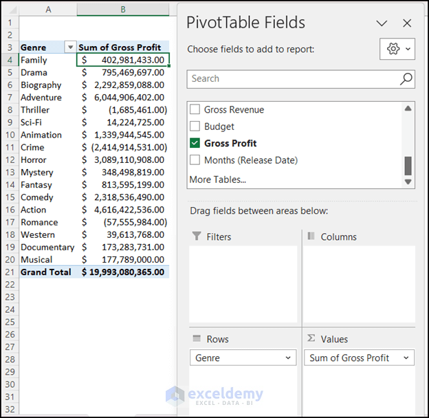
Dear Yosh,
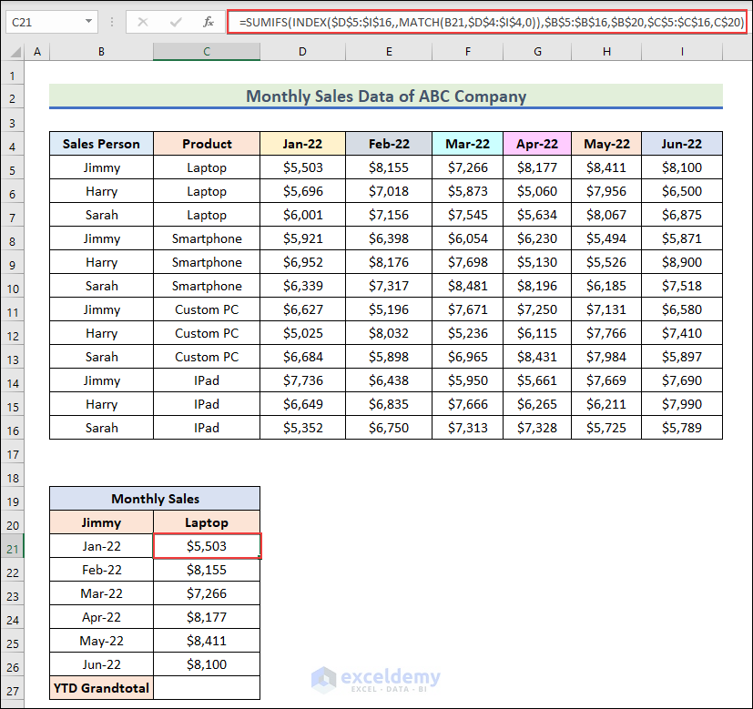
Thank you for your query. Yes, you can determine the sum of YTD number. Firstly create a table like the following for each Month’s Sales of “Jimmy” for “Laptop”.
Copy this formula in cell C21.
=SUMIFS(INDEX($D$5:$I$16,,MATCH(B21,$D$4:$I$4,0)),$B$5:$B$16,$B$20,$C$5:$C$16,C$20)

You will get the sales for each month.
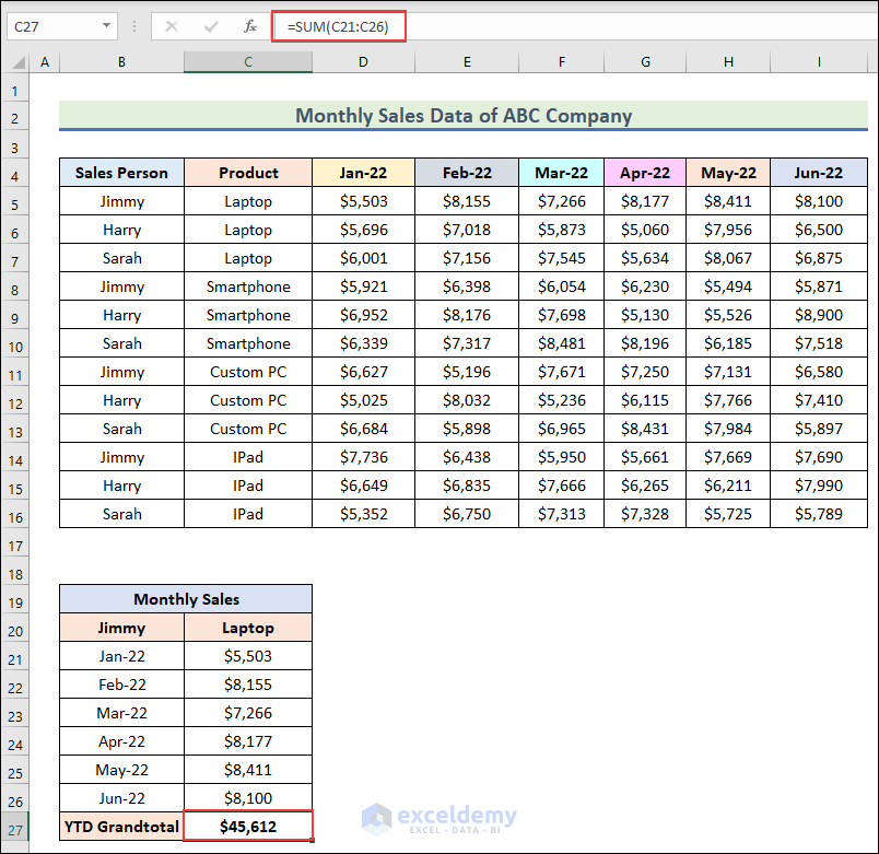
Next, to calculate the “YTD Grandtotal” copy this formula in cell C27.
=SUM(C21:C26)

I hope this method will solve your problem. Thank you!
Mahfuza Anika Era
ExcelDemy
Reply
Mahfuza Anika Era Jul 25, 2023 at 12:13 PM

Dear Yosh,
I assume, this question is same as the previous one. You can follow the steps I have given in the previous reply. If you still have any confusion, please leave a comment describing your problem. Thank you!
Mahfuza Anika Era
ExcelDemy
Reply
Mahfuza Anika Era May 14, 2023 at 5:12 PM

Dear L,
Thank you for your comment. This formula calculates a date value. Here is a breakdown of what each part of the formula does:

=$B$4-(WEEKDAY(C$3,1)-($AM$7-1))-IF((WEEKDAY($B$4,1)-($AM$7-1))<=0,7,0)+1

$B$4: This is the reference to cell B4 which contains the date value you enter in Customize Dates Table.
WEEKDAY(C$3,1): This function calculates the weekday of the date in cell C3. The argument 1 specifies that the weekday numbering should start on Monday (1) instead of Sunday (default value of 0).
$AM$7: This is a reference to the cell containing a number that specifies the Start Month. (e.g. 1 for Monday, 7 for Sunday).
IF((WEEKDAY($B$4,1)-($AM$7-1))<=0,7,0): This function checks whether the weekday of the date in cell B4 is earlier in the week than the specified start day of the week. If it is, the function returns 7 (the number of days in a week) to adjust the date calculation later. If not, the function returns 0.
B4-(WEEKDAY(C3,1)-($AM$7-1))-IF((WEEKDAY($B$4,1)-($AM$7-1))<=0,7,0)+1: This formula subtracts the weekday of the date in cell C3 from the date in cell B4, then adds the start day of the week minus 1, and finally subtracts the result of the IF function. This calculates the first day of the week that contains the date in cell B4. The final +1 adds one day to get the actual start date of the week.
If you want 4 weeks in one sheet, just add 3 more weeks similarly in the existing sheet. Hope this will help you.
Regards
Mahfuza Anika Era
ExcelDemy

Mahfuza Anika Era May 11, 2023 at 4:51 PM

Dear Max,
Thank you for your query. Changing the currency is not the reason behind the incorrect output of the module 2 code. Actually, the code is not working for the last 3 digits of the whole number part. Here is the modified code of module 1 that may help you. This will give the correct result hopefully.

Function number_converting_into_currency(ByVal MyNumber)
Dim x_string As String
Dim whole_num As Integer
Dim x_string_pnt
Dim x_string_Num
Dim x_pnt As String
Dim x_numb As String
Dim x_P() As Variant
Dim x_DP
Dim x_cnt As Integer
Dim x_output, x_T As String
Dim x_my_len As Integer
On Error Resume Next
x_P = Array("", "Thousand ", "Million ", "Billion ", "Trillion ", " ", " ", " ", " ")
x_numb = Trim(Str(MyNumber))
x_DP = InStr(x_numb, ".")
x_pnt = ""
x_string_Num = ""
If x_DP > 0 Then
x_pnt = " "
x_string = Mid(x_numb, x_DP + 1)
x_string_pnt = Left(x_string, Len(x_numb) - x_DP)
For whole_num = 1 To Len(x_string_pnt)
x_string = Mid(x_string_pnt, whole_num, 1)
x_pnt = x_pnt & get_digit(x_string) & " "
Next whole_num
x_numb = Trim(Left(x_numb, x_DP - 1))
End If
x_cnt = 0
x_output = ""
x_T = ""
x_my_len = 0
x_my_len = Int(Len(Str(x_numb)) / 3)
If (Len(Str(x_numb)) Mod 3) = 0 Then x_my_len = x_my_len - 1
Do While x_numb <> ""
If x_my_len = x_cnt Then
x_T = get_hundred_digit(Right(x_numb, 3), False)
Else
If x_cnt = 0 Then
x_T = get_hundred_digit(Right(x_numb, 3), True)
Else
x_T = get_hundred_digit(Right(x_numb, 3), False)
End If
End If
If x_T <> "" Then
x_output = x_T & x_P(x_cnt) & x_output
End If
If Len(x_numb) > 3 Then
x_numb = Left(x_numb, Len(x_numb) - 3)
Else
x_numb = ""
End If
x_cnt = x_cnt + 1
Loop
If x_DP > 0 Then
x_output = x_output & "dollars" & x_pnt & "Cents"
Else
x_output = x_output & "dollars"
End If
number_converting_into_currency = x_output
End Function
Function get_hundred_digit(xHDgt, y_b As Boolean)
Dim x_R_str As String
Dim x_string_Num As String
Dim x_string As String
Dim y_I As Integer
Dim y_bb As Boolean
x_string_Num = xHDgt
x_R_str = ""
On Error Resume Next
y_bb = True
If Val(x_string_Num) = 0 Then Exit Function
x_string_Num = Right("000" & x_string_Num, 3)
x_string = Mid(x_string_Num, 1, 1)
If x_string <> "0" Then
x_R_str = get_digit(Mid(x_string_Num, 1, 1)) & "Hundred "
Else
If y_b Then
x_R_str = "and "
y_bb = False
Else
x_R_str = " "
y_bb = False
End If
End If
If Mid(x_string_Num, 2, 2) <> "00" Then
x_R_str = x_R_str & get_ten_digit(Mid(x_string_Num, 2, 2), y_bb)
End If
get_hundred_digit = x_R_str
End Function
Function get_ten_digit(x_TDgt, y_b As Boolean)
Dim x_string As String
Dim y_I As Integer
Dim x_array_1() As Variant
Dim x_array_2() As Variant
Dim x_T As Boolean
x_array_1 = Array("Ten ", "Eleven ", "Twelve ", "Thirteen ", "Fourteen ", "Fifteen ", "Sixteen ", "Seventeen ", "Eighteen ", "Nineteen ")
x_array_2 = Array("", "", "Twenty ", "Thirty ", "Forty ", "Fifty ", "Sixty ", "Seventy ", "Eighty ", "Ninety ")
x_string = ""
x_T = True
On Error Resume Next
If Val(Left(x_TDgt, 1)) = 1 Then
y_I = Val(Right(x_TDgt, 1))
If y_b Then x_string = "and "
x_string = x_string & x_array_1(y_I)
Else
y_I = Val(Left(x_TDgt, 1))
If Val(Left(x_TDgt, 1)) > 1 Then
If y_b Then x_string = "and "
x_string = x_string & x_array_2(Val(Left(x_TDgt, 1)))
x_T = False
End If
If x_string = "" Then
If y_b Then
x_string = " "
End If
End If
If Right(x_TDgt, 1) <> "0" Then
x_string = x_string & get_digit(Right(x_TDgt, 1))
End If
End If
get_ten_digit = x_string
End Function
Function get_digit(xDgt)
Dim x_string As String
Dim x_array_1() As Variant
x_array_1 = Array("Zero ", "One ", "Two ", "Three ", "Four ", "Five ", "Six ", "Seven ", "Eight ", "Nine ")
x_string = ""
On Error Resume Next
x_string = x_array_1(Val(xDgt))
get_digit = x_string
End Function

Copy the code in your module and Run the code.

I hope you have got your problem solved. Thank you.
Regards
Mahfuza Anika Era
ExcelDemy