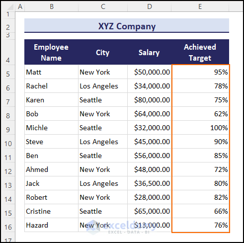
Returning all rows that match criteria in Excel means showing the rows in a dataset that meet specific conditions. For example, this is a dataset showing employee details of a company. We want to return the rows from this dataset based on the City name, specifically New York.
Method 1 – Using Excel Formula to Return All Rows That Match Criteria in Excel
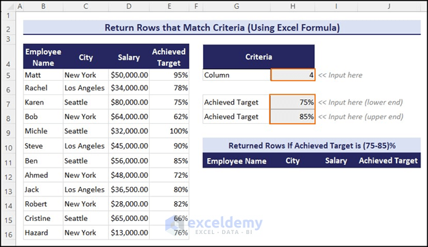
The following dataset represents the employee details of a company. Here, the column Achieved Target shows the performance of the employees. We want to return the rows based on the value of the Achieved Target column.
Steps:
- Create a Criteria table like the following one.
- Enter the lower and upper end of the criteria values of the Target Achieved column. Here, Column indicates the column number where your criteria is located.
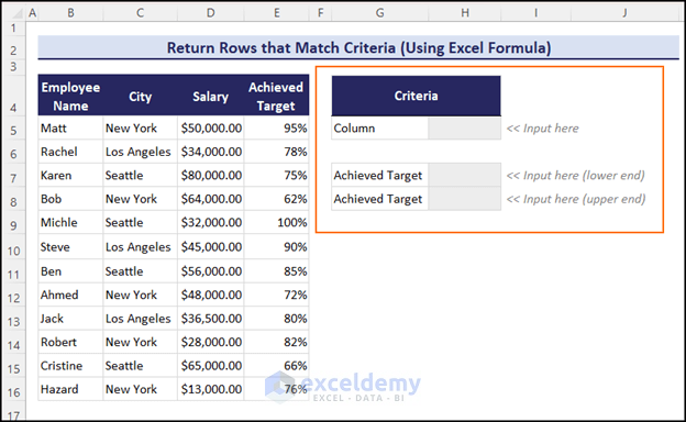
- Create another table with the same headings as the original dataset.
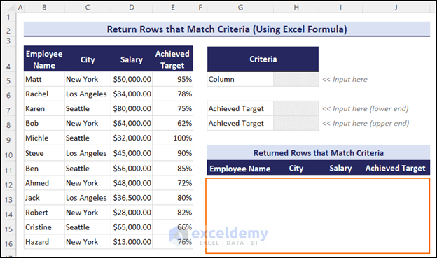
- Input the criteria.
Here, we want to return the rows based on Achieved Target. Now, the Achieved Target column is column number 4 in our dataset. So, in Column field, we will insert 4. Input the lower-end and upper-end criteria value of the Achieved Target. Here, we want to return the rows where the Achieved Target is between 75-85%.
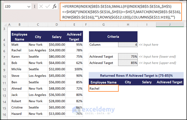
- Write this formula in cell G11 and press the Enter key:
=IFERROR(INDEX($B$5:$E$16,SMALL(IF((INDEX($B$5:$E$16,,$H$5)<=$H$8)*(INDEX($B$5:$E$16,,$H$5)>=$H$7),MATCH(ROW($B$5:$E$16),ROW($B$5:$E$16)),""),ROWS(G12:$G$12)),COLUMNS($E$11:E11)),"")The formula will return the value Rachel which is the value in the Employee Name column. The Achieved Target of Rachel is 78% and it is between 75-85%, making it the first hit in the table.
=IFERROR(INDEX($B$5:$E$16,SMALL(IF((INDEX($B$5:$E$16,,$H$7)<=$H$6)*(INDEX($B$5:$E$16,,$H$7)>=$H$5),MATCH(ROW($B$5:$E$16),ROW($B$5:$E$16)),””),ROWS(G11:$G$11)),COLUMNS($F$11:F11)),””)
=IFERROR(INDEX($B$5:$E$16,SMALL(IF((INDEX($B$5:$E$16,,$H$7)<=$H$6)*(INDEX($B$5:$E$16,,$H$7)>=$H$5),MATCH(ROW($B$5:$E$16),ROW($B$5:$E$16)),””),ROWS(G11:$G$11)),1),””)// COLUMNS($F$11:F11) returns 1 because the count of column is 1 in the given range.
=IFERROR(INDEX($B$5:$E$16,SMALL(IF((INDEX($B$5:$E$16,,$H$7)<=$H$6)*(INDEX($B$5:$E$16,,$H$7)>=$H$5),MATCH(ROW($B$5:$E$16),ROW($B$5:$E$16)),””),1),1),””) // ROWS(G11:$G$11) returns 1 because the count of rows is 1 in the given range.
=IFERROR(INDEX($B$5:$E$16,SMALL(IF((INDEX($B$5:$E$16,,$H$7)<=$H$6)*(INDEX($B$5:$E$16,,$H$7)>=$H$5),MATCH(ROW($B$5:$E$16),{5;6;7;8;9;10;11;12;13;14;15;16}),””),1),1)””) // ROW($B$5:$E$16) returns the array {5;6;7;8;9;10;11;12;13;14;15;16} which are the row numbers.
=IFERROR(INDEX($B$5:$E$16,SMALL(IF((INDEX($B$5:$E$16,,$H$7)<=$H$6)*(INDEX($B$5:$E$16,,$H$7)>=$H$5),MATCH({5;6;7;8;9;10;11;12;13;14;15;16},{5;6;7;8;9;10;11;12;13;14;15;16}),””),1),1),””) // ROW($B$5:$E$16) returns the array {5;6;7;8;9;10;11;12;13;14;15;16} which are the row numbers.
=IFERROR(INDEX($B$5:$E$16,SMALL(IF((INDEX($B$5:$E$16,,$H$7)<=$H$6)*(INDEX($B$5:$E$16,,$H$7)>=$H$5),{1;2;3;4;5;6;7;8;9;10;11;12},””),1),1),””)
// MATCH({5;6;7;8;9;10;11;12;13;14;15;16},{5;6;7;8;9;10;11;12;13;14;15;16}) returns {1;2;3;4;5;6;7;8;9;10;11;12} because these are the relative positions.
=IFERROR(INDEX($B$5:$E$16,SMALL(IF((INDEX($B$5:$E$16,,$H$7)<=$H$6)*({0;0.95;0.78;0.75;0.62;1;0.9;0.85;0.72;0.8;0.82;0.66}>=$H$5),{1;2;3;4;5;6;7;8;9;10;11;12},””),1),1),””) // (INDEX($B$5:$E$16,,$H$7) returns {0;0.95;0.78;0.75;0.62;1;0.9;0.85;0.72;0.8;0.82;0.66} as these are the reference values it gets.
=IFERROR(INDEX($B$5:$E$16,SMALL(IF(({0;0.95;0.78;0.75;0.62;1;0.9;0.85;0.72;0.8;0.82;0.66}<=$H$6)*({0;0.95;0.78;0.75;0.62;1;0.9;0.85;0.72;0.8;0.82;0.66}>=$H$5),{1;2;3;4;5;6;7;8;9;10;11;12},””),1),1),””) // INDEX($B$5:$E$16,,$H$7) returns the reference array {0;0.95;0.78;0.75;0.62;1;0.9;0.85;0.72;0.8;0.82;0.66}.
=IFERROR(INDEX($B$5:$E$16,SMALL({“”;2;””;””;””;6;7;8;””;10;11;””},1),1),””) // IF(({0;0.95;0.78;0.75;0.62;1;0.9;0.85;0.72;0.8;0.82;0.66}<=$H$6)*({0;0.95;0.78;0.75;0.62;1;0.9;0.85;0.72;0.8;0.82;0.66}>=$H$5),{1;2;3;4;5;6;7;8;9;10;11;12},””) gives {“”;2;””;””;””;6;7;8;””;10;11;””} because it returns the row numbers where the IF conditions match and returns “” if it doesn’t match.
=IFERROR(INDEX($B$5:$E$16,2,1),””) // SMALL({“”;2;””;””;””;6;7;8;””;10;11;””},1) returns 2 as the smallest row number. It is to show the values sequentially.
=IFERROR(Matt,””) // INDEX($B$5:$E$16,2,1) returns the value Matt as it is situated at the intersection of the first column and second row of the B5:E16 range.
=Matt // IFERROR(Matt,””) returns Matt as it didn’t find any error. If an error occurs it will return blank.
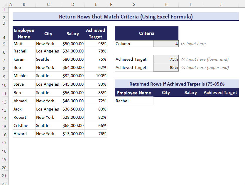
- Hover over the bottom-right corner of the cell G12. The cursor will be changed to the Fill Handle feature.
- Drag the Fill Handle vertically and horizontally to AutoFill the formulas until you get blank cells.
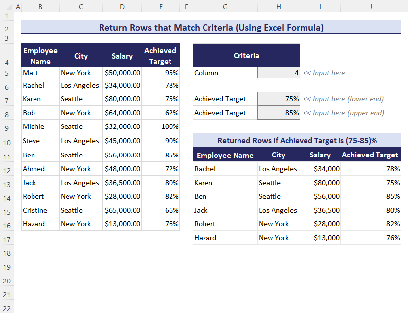
Thus, you will get all the rows where the value of the Achieved Target column is between 75-85%.
Since the table is dynamic, you can enter any values for Achieved Target in the criteria table and it will return the rows.
Note: In this table, we applied conditional formatting in Salary and Achieved Target columns, we have used conditional formatting. The rule is if the cells are non-blank, the Salary column will be in Currency format and the Achieved Target column will be in Percentage format.
We don’t know how many rows will return that match the criteria. So, we have applied a new rule in range G12:J24 that if the cells are non-blank border will be added. As a result, the returned rows that match criteria will be bordered automatically.
Method 2 – Using Excel’s Filter Button in Excel Table to Return All Rows That Match Criteria
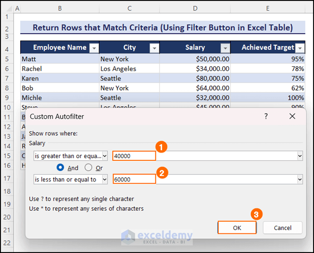
This time, we’ll filter the rows based on the Salary column. We want to filter the rows where the salary of the employees is in between $40,000-$60,000 range.
Steps:
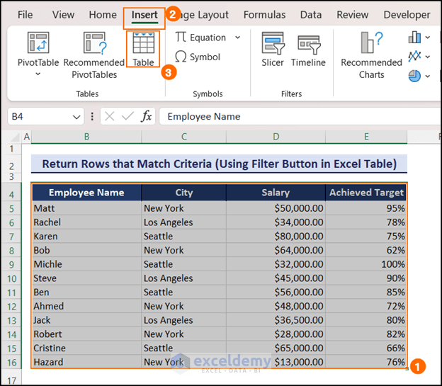
- Select the entire dataset.
- Go to the Insert tab and Tables group.
- Click on the Table option.
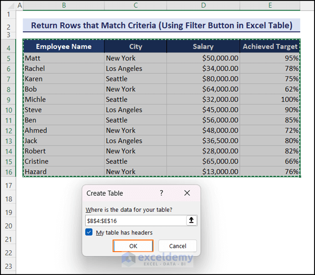
- A Create Table dialog box will appear.
- Under the Where is the data for your table? field, the selected range will be shown.
- As we selected the range including the header, keep the My table has headers option checked.
- Press the OK button.
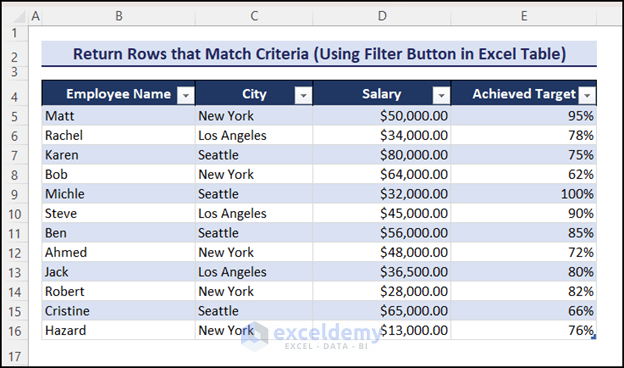
- Excel will convert our dataset into a table.
- Select the down arrow icon at the bottom-right corner of the Salary header.
- Click on the Number Filters option and select the Between option.
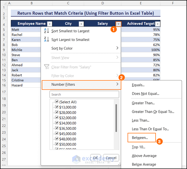
- A Custom Autofilter dialog box will appear.
- Beside the is greater than or equal to field, enter the minimum range which is 40000.
- Beside the is less than or equal to field, enter the maximum range which is 60000.
- Hit the OK button.
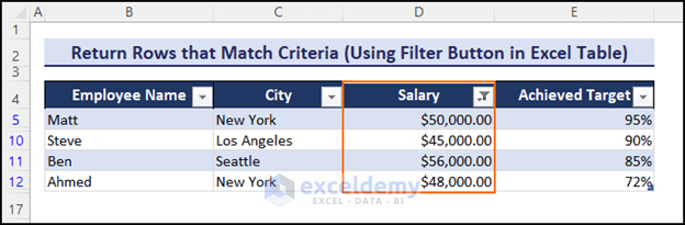
- You will get the rows where the value of the Salary column is in the 40,000-60,000 range. You can see a filter icon at the bottom-right corner of the column based on which you filtered the rows.
Note: The Filter button temporarily modifies the table. You can clear the filters from the Data tab, Sort and Filter group of commands option Clear.
Method 3 – Using Excel’s Advanced Filter Feature
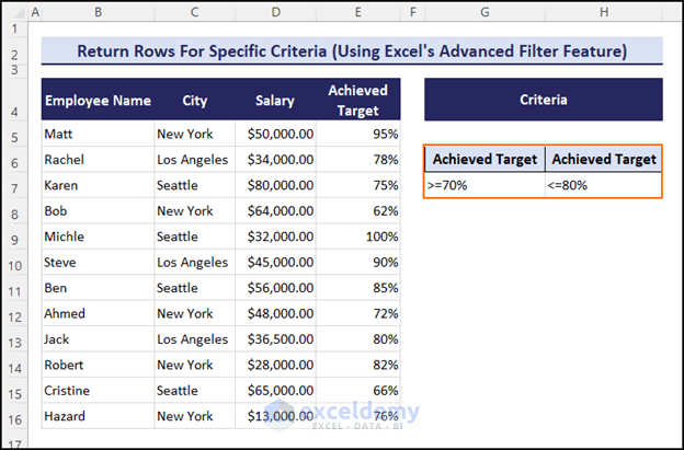
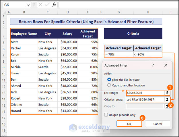
This time, we want to return the rows where the Achieved Target is between 70-80%.
Steps:
- Create a table to define your criteria. We want to return rows based on the Achieved Target column. So, we created the table by defining the values of Achieved Target. It is >=70% and <=80%.
Note: Be careful about the spelling of the headers of the criteria table. The column headers of the criteria table must match exactly with the dataset table. Otherwise, the Advanced Filter won’t detect the column where it will apply the filter.
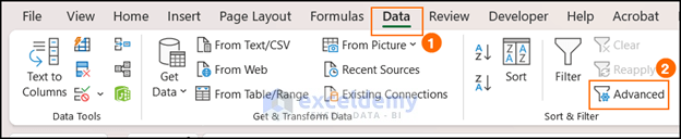
- Click on the Data tab and go to the Sort & Filter group.
- Select the Advanced option right beside the Filter command.
- The Advanced Filter dialog box will appear.
- In the List range field, select the range of the entire dataset including the headings. For our dataset, it is B4:E16.
- In the Criteria range field, select the range of the criteria table including the headings. It’s G6:H7 for this dataset.
- Click on the OK button.
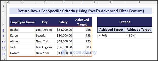
You will get the rows where the Achieved Targets of the employees are between 70-80%.
Note: The Advanced Filter option temporarily modifies the table. You can clear the filters from the Data tab => Sort and Filter group of commands =>Clear option.
Method 4 – Using FILTER Function to Return All Rows That Match Criteria in Excel
The FILTER function is only available in Excel 365.
Case 4.1 Based on Single Criteria
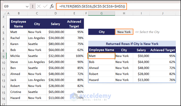
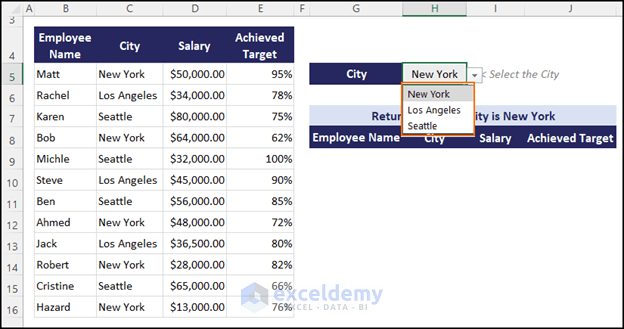
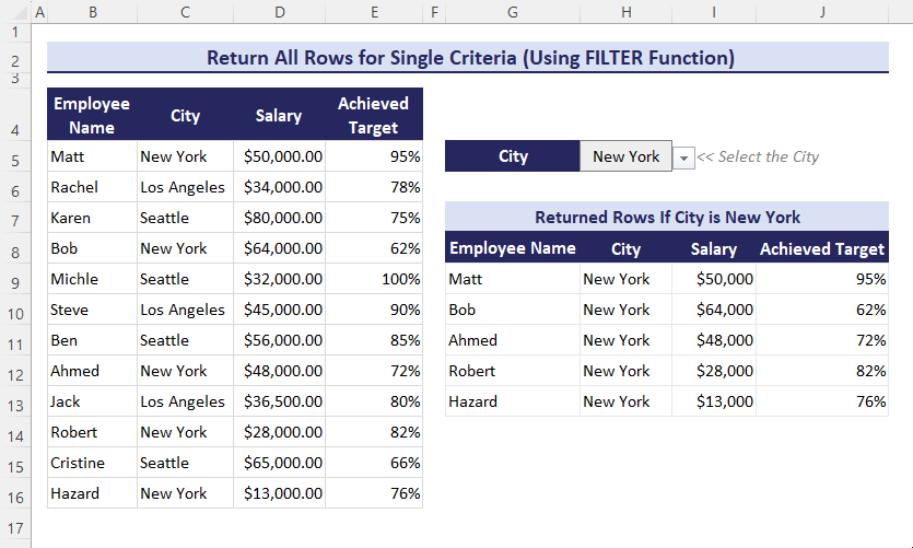
In our dataset, we want to return the rows based on single criteria. Here our criteria is the City column.
Note: We have used the Data Validation tool in cell H5. You can choose a specific city from here. If you choose New York, the FILTER function will return the rows where the city name is New York.
Steps:
- Enter this formula in cell G9 and press Enter:
=FILTER($B$5:$E$16,($C$5:$C$16=$H$5))Thus, you will get all rows where the City is New York. The FILTER function returns the array from B5:E16 range if the range C5:C16 matches with the value of H5 cell.

- Select the City in cell H5, you will get the rows automatically.
Note: If there are not enough empty cells available for the output data of the FILTER function, it’ll give #SPILL!
Case 4.2 Based on Multiple Criteria
Submethod 1 – Using the FILTER Function
In this dataset, we want to return the rows where the value of the Achieved Target is.
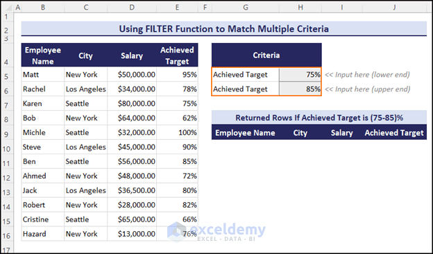
Steps:
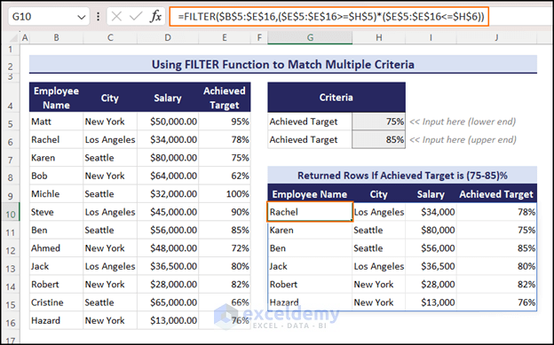
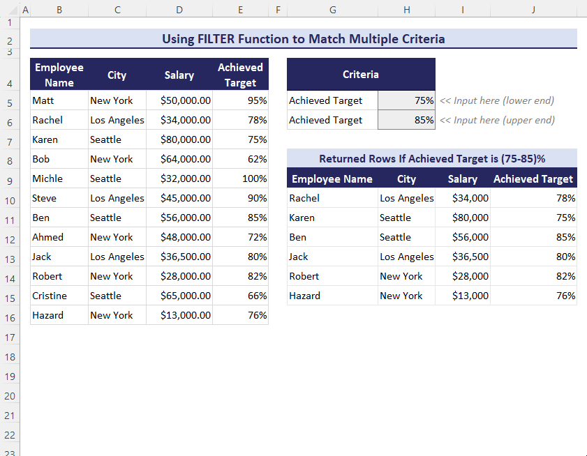
- Write this formula in cell G10 and press the Enter key.
=FILTER($B$5:$E$16,($E$5:$E$16>=$H$5)*($E$5:$E$16<=$H$6))You will get the rows where the value of the Achieved Target column is between the 75-85% range.
=FILTER($B$5:$E$16,($E$5:$E$16>=$H$5)*($E$5:$E$16<=$H$6))
=FILTER($B$5:$E$16,($E$5:$E$16>=$H$5)*{TRUE;TRUE;TRUE;TRUE;TRUE;TRUE;TRUE;TRUE;TRUE;TRUE;TRUE;TRUE}) // ($E$5:$E$16<=$H$6) this part checks if the range E5:E16 is less than or equal to cell H6. If it matches, it returns TRUE. Otherwise, it returns FALSE.
=FILTER($B$5:$E$16,{TRUE;FALSE;FALSE;FALSE;TRUE;TRUE;TRUE;FALSE;TRUE;TRUE;FALSE;FALSE}*{TRUE;TRUE;TRUE;TRUE;TRUE;TRUE;TRUE;TRUE;TRUE;TRUE;TRUE;TRUE}) // ($E$5:$E$16>=$H$5) checks if the range E5:E16 is greater than or equal to cell H6. If it matches, it returns TRUE. Otherwise, it returns FALSE.
{“Matt”,”New York”,50000,0.95;”Michle”,”Seattle”,32000,1;”Steve”,”Los Angeles”,45000,0.9;”Ben”,”Seattle”,56000,0.85;”Jack”,”Los Angeles”,36500,0.8;”Robert”,”New York”,28000,0.82} // =FILTER($B$5:$E$16,{TRUE;FALSE;FALSE;FALSE;TRUE;TRUE;TRUE;FALSE;TRUE;TRUE;FALSE;FALSE}*{TRUE;TRUE;TRUE;TRUE;TRUE;TRUE;TRUE;TRUE;TRUE;TRUE;TRUE;TRUE}) returns the array where both conditions are TRUE.
The rows will return according to your given input in the criteria table.
Submethod 2 – Combining FILTER and COUNTIF Functions
Here, we want to get the rows based on two cities. We have applied the Data Validation tool in the G5:G6 range.
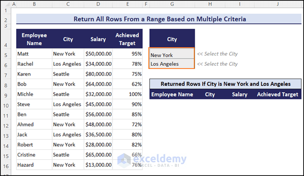
- Write this formula in cell G10.
=FILTER($B$5:$E$16, COUNTIF($G$5:$G$6, $C$5:$C$16))- Press the Enter key and you will get the rows where the City is New York and Los Angeles.
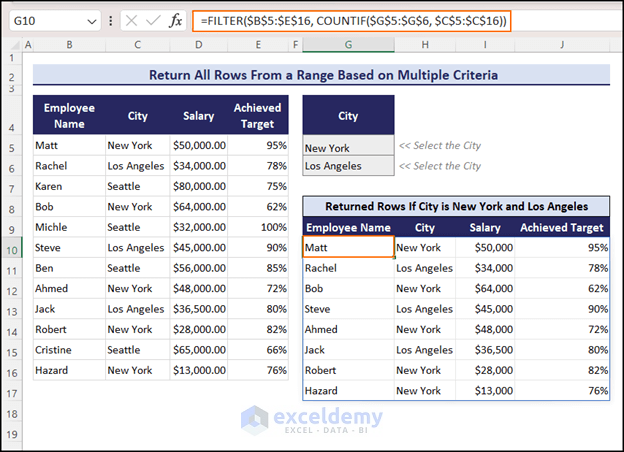
=FILTER($B$5:$E$16, COUNTIF($G$5:$G$6, $C$5:$C$16))
=FILTER($B$5:$E$16, {1;1;0;1;0;1;0;1;1;1;0;1})// COUNTIF($G$5:$G$6, $C$5:$C$16) returns {1;1;0;1;0;1;0;1;1;1;0;1} because it returns 1 if it matches the value with $G$5:$G$6 range. Otherwise, it returns 0.
{“Matt”,”New York”,50000,0.95;”Rachel”,”Los Angeles”,34000,0.78;”Bob”,”New York”,64000,0.62;”Steve”,”Los Angeles”,45000,0.9;”Ahmed”,”New York”,48000,0.72;”Jack”,”Los Angeles”,36500,0.8;”Robert”,”New York”,28000,0.82;”Hazard”,”New York”,13000,0.76}// FILTER($B$5:$E$16, {1;1;0;1;0;1;0;1;1;1;0;1}) returns the array based on the criteria of the COUNTIF function.
Since this formula is dynamic, the returned rows will change according to your given cities.
Download Practice Workbook
<< Go Back to | Excel Match | Learn Excel
Get FREE Advanced Excel Exercises with Solutions!
