Method 1 – Use the IF Function to Check If One Cell Equals Another and Return Another Value
Case 1.1 – Returning the Exact Value of Cell
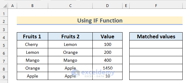
We have a dataset of some Fruits with two columns. Every row has a specific Value. We will find the rows where Fruits 1 and Fruits 2 are matched and display the Value in the Matched Values column.
Steps:
- Enter the following formula in cell F5.
=IF(B5=C5,D5,"")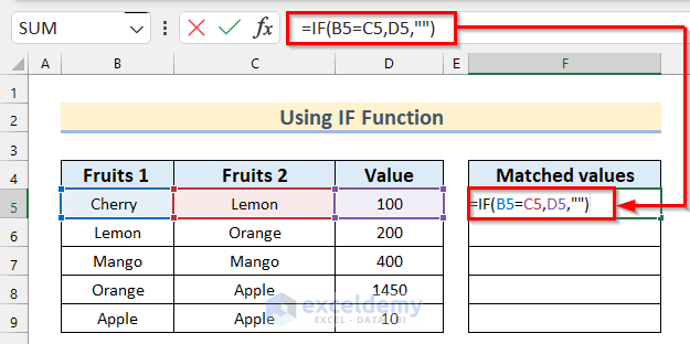
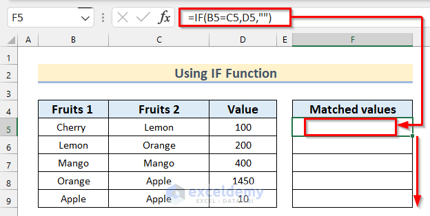
- Press Enter.
- Drag down the Fill Handle tool to AutoFill the formula for the rest of the cells.
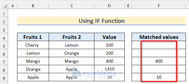
- Here’s the result.
Case 1.2 – Updating the Resulting Value
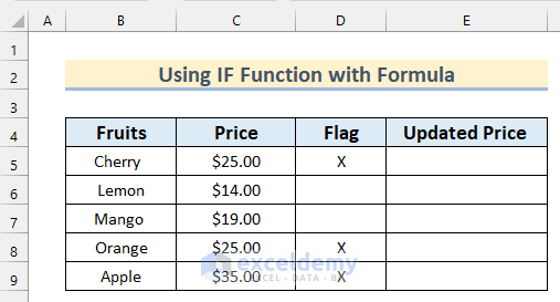
We will update the new Price if the Flag value is not X, where the new price will be 2 times the current price.
Steps:
- Enter the following formula in cell E5.
=IF(D5<>"X",C5*2,C5)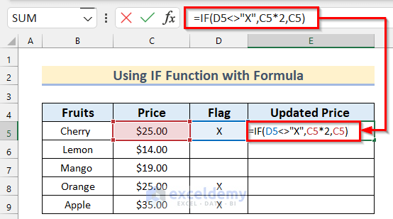
- Press Enter and copy down the formula to cell E9.
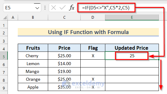
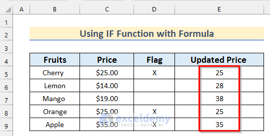
- Here’s the result.
Method 2 – Return Another Cell Value Using the VLOOKUP Function
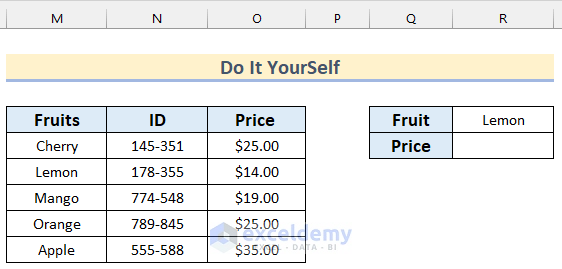
Consider a dataset of some Fruits. We have 3 columns: Fruits, ID, and Price. We will search for specific fruit prices from this table.

Steps:
- Enter the following formula in cell G5.
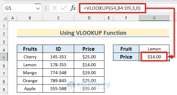
=VLOOKUP(G4,B4:D9,3,0)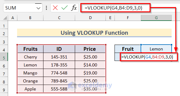
- Press Enter.
- You can find any other Fruit’s price by entering its Name on Cell G4.
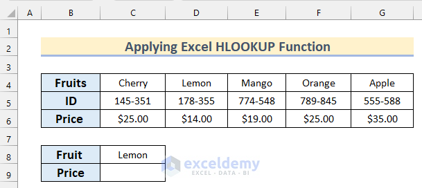
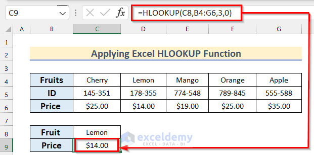
Method 3 – Apply the HLOOKUP Function to Scan for a Matching Value
The syntax of the HLOOKUP functions is:
=HLOOKUP (lookup_value, table_array, row_index, [range_lookup])We have swapped the rows and columns to show the function.
Steps:
- Select cell C9 and insert the following formula.
=HLOOKUP(C8,B4:G6,3,0)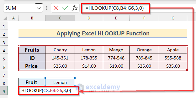
- Press Enter.
Method 4 – Check If One Cell Equals Another with INDEX and MATCH Functions
Steps:
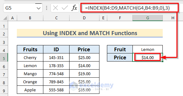
- Enter the following formula in cell G5.
=INDEX(B4:D9,MATCH(G4,B4:B9,0),3)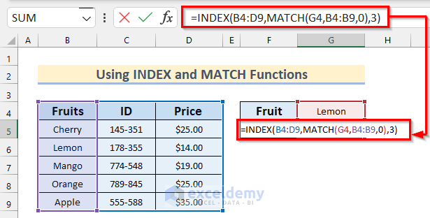
- Press Enter.
Method 5 – Return Items from Another Worksheet with Matching Value in Excel
We have two worksheets, Weekly Meals and Ingredients. We’ll compare meals and show the ingredients in the first worksheet. The Week Meals Planning worksheet looks like the following:
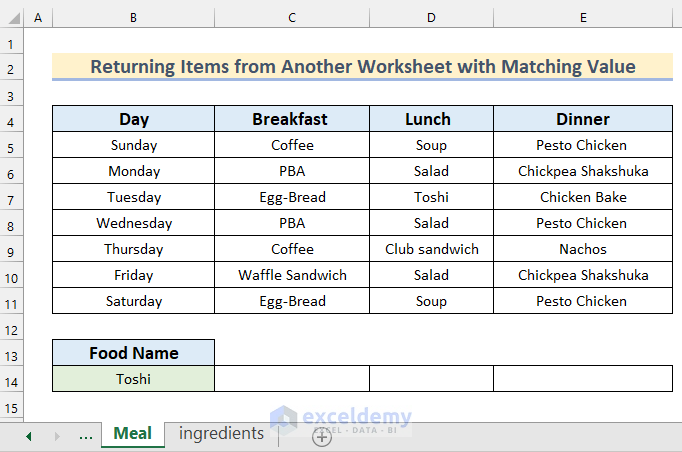
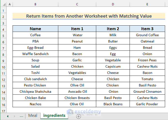
Here’s the Ingredients sheet. We’ll find the food ingredients from this worksheet by entering the name of the food in cell B14 in the Meals sheet.
Steps:
- Enter this formula in cell C14.
=VLOOKUP($B14,ingredients!$B$5:$E$16,COLUMN()-1,FALSE)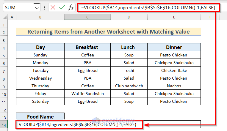
- Press Enter.
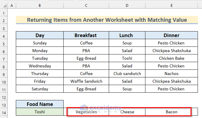
- Copy the formula to the right.
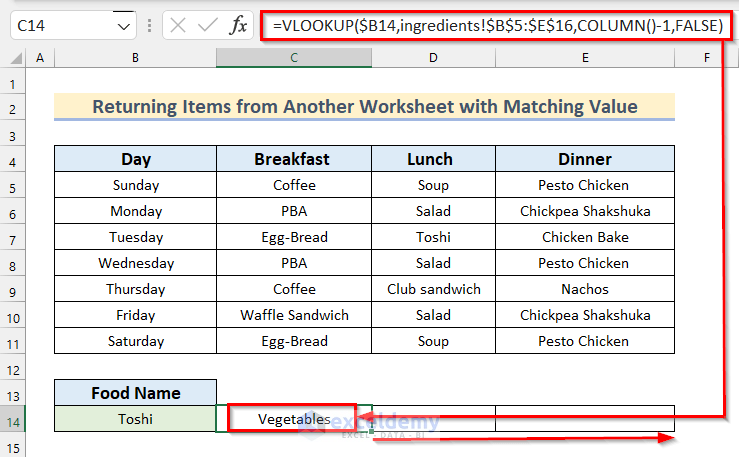
- All the ingredients of the selected Food will be displayed.
Practice Section
In the download file, you will find an Excel workbook like the image given below to practice on your own.
Download the Practice Workbook
<< Go Back to | Excel Match | Learn Excel
Get FREE Advanced Excel Exercises with Solutions!

Dear Mr Abdullah Al Murad,
I have read your examples with great interest. I have used the example above with INDEX and MATCH to retrieve a value from an Excel sheet of information by using a drop down list to choose the value I want to search for.
=INDEX(Total!A3:G33, MATCH(Testing!$B$2, Total!D3:D33, 0), 1)
The sheet Total contains a number of rows and columns of information, where column D contains years (one year or several comma separated) and column E months (one or several comma separated). Testing!B2 contains a list of years 2021-2031 where I can choose a specific year from the drop down list, and Testing!D2 contains months.
What I really would do is to expand this in three ways. The use case being that as a user I would be able to retrieve specific rows from the sheet Total by choosing the year and month of interest and displaying them in the sheet Testing.
Firstly I would like to retrieve all lines from the table of information that matches the input criteria. So if I choose 2025, all lines containing 2025 should be listed below where I choose from the drop down.
Secondly I would like to choose the lines containing the year even if there are several years in the data. So if the cell Total!D5 contains “2025” or “2025, 2026, 2027” the row should be presented in the result.
Thirdly I want to add a second criteria. I want to be able to choose both year and month from two separate drop downs. So if Testing!B2 is 2025 and Total!D3:D33 contains 2025, or the Testing!E2 contains January (or e.g. January, February) and Total!E3:E33 contains January I should get all rows containing either 2025 or January.
I hope you can help me with this as I think this is probably easy for you 🙂 I have been programming PERL and Java but to implement algorithms with the functions in Excel is a bit beyond me.
Thank you for a very good instructional site on Excel!
Thanks a lot OSCAR APPELGREN for your questions.
In response to your first question to have matched rows entirely in the drop-down, it is not possible in Excel. A standard drop-down list in Excel does not support multiple rows of data.
If you want to filter multiple rows based on single or multiple criteria, you better use the FILTER function. It is not applicable to the older Excel version. It helps you to extract multiple matched rows quite easily than INDEX-MATCH functions.
According to your requirements to extract matched rows based on single criteria (i.e. year 2025), I have used the following formula which works pretty well.
=FILTER(B3:E17,D3:D17=H4)
And, for sorting rows with multiple criteria, you just need to use the asterisk sign(*) and insert the other condition.
=FILTER(B3:E17,(D3:D17=H4)*(E3:E17=H5))
Fantastic, thank you! Just what I needed.
Dear Aspen,
You are most welcome.
Regards
ExcelDemy