Overview
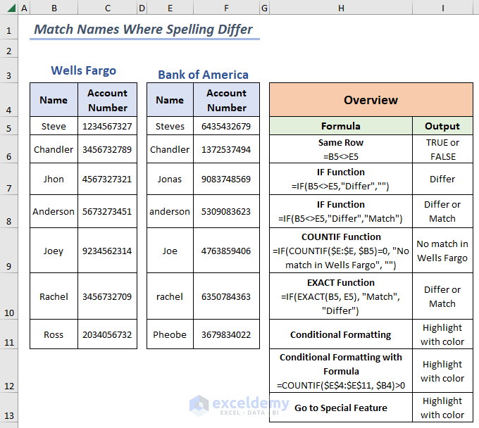
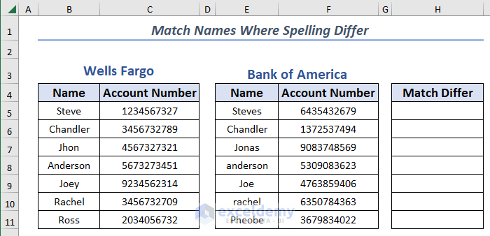
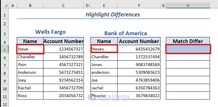
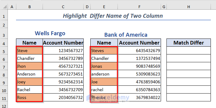
The sample dataset contains Name and Account Number of the same person in different banks.
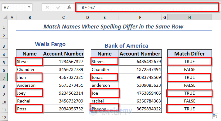
Method 1 – Matching Names with different Spelling in the Same Row
- Select the cell to place the result. Here, H5.
- Enter formula.
=B5<>E5
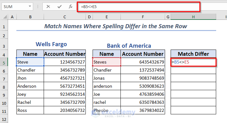
- Press ENTER.
- If the value of different columns but the same row differs, it returns True. Otherwise, False
- In the Match Differ column, it will show TRUE as B5 and E5 were selected.
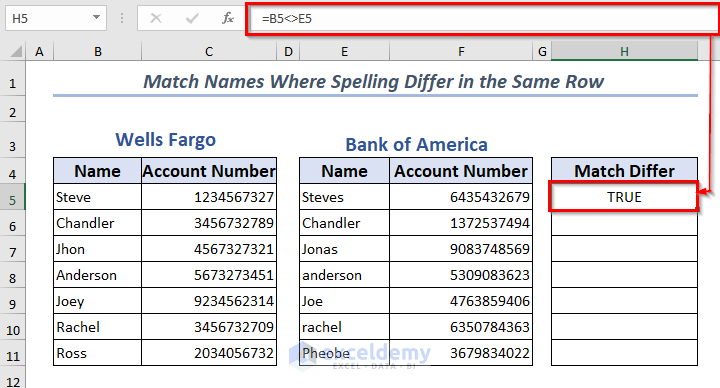
- Drag the Fill Handle to AutoFill the rest of the cells in the column.
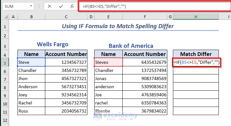
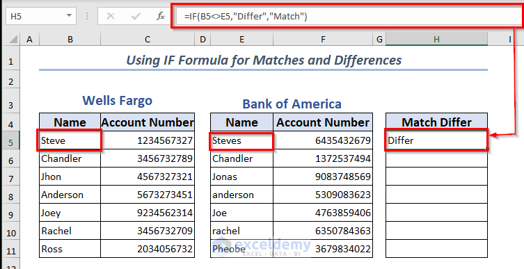
Method 2 – Using the IF Formula to Match Spelling Differences
- Select a cell to place your resultant value. Here, H5.
- Enter the formula.
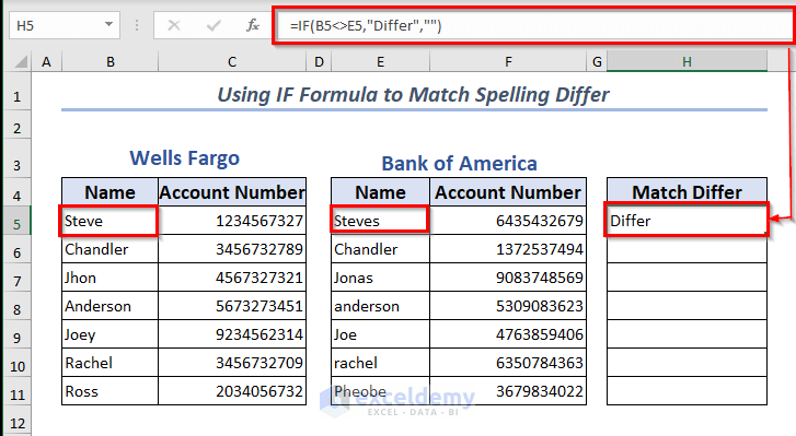
=IF(B5<>E5,"Differ","")
- Press ENTER.
- It will return Differ when the compared names’ spelling is different. If spelling matches it will keep the cell empty.
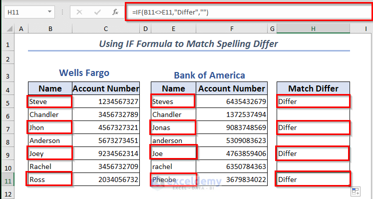
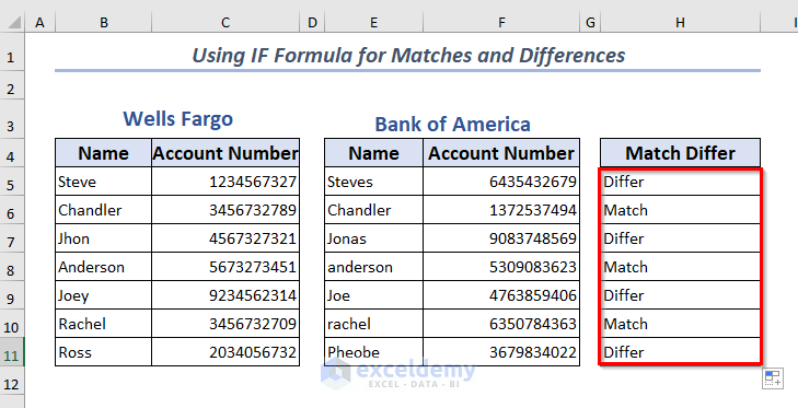
- Drag the Fill Handle to AutoFill the rest of the cells in the column.
Method 3 – Using the IF Formula for Both Matches and Differences
- Select H5 cell to enter the formula.
=IF(B5<>E5,"Differ","Match")
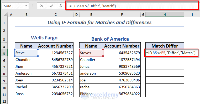
- Press ENTER.
- It will return either Differ or Match.
- Drag the Fill Handle to AutoFill the rest of the cells in the column.
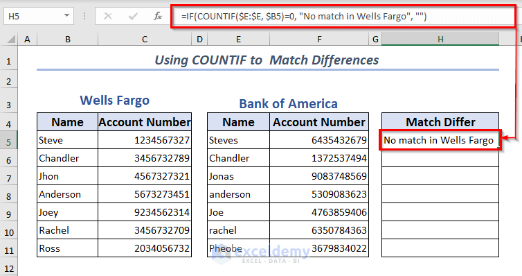
Method 4 – Using the COUNTIF to Match Differences
- Select a cell to enter the formula. Here, H5.
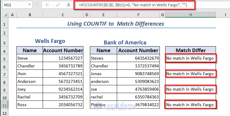
=IF(COUNTIF($E:$E, $B5)=0, "No match in Wells Fargo", "")
-
- The name in B5 is compared with the names in Column E .
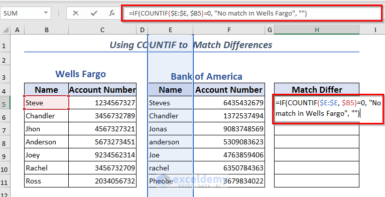
- Press ENTER.
- It will show No match in Wells Fargo if the spelling differs from Bank of America.
- Drag the Fill Handle to AutoFill the rest of the cells in the column.
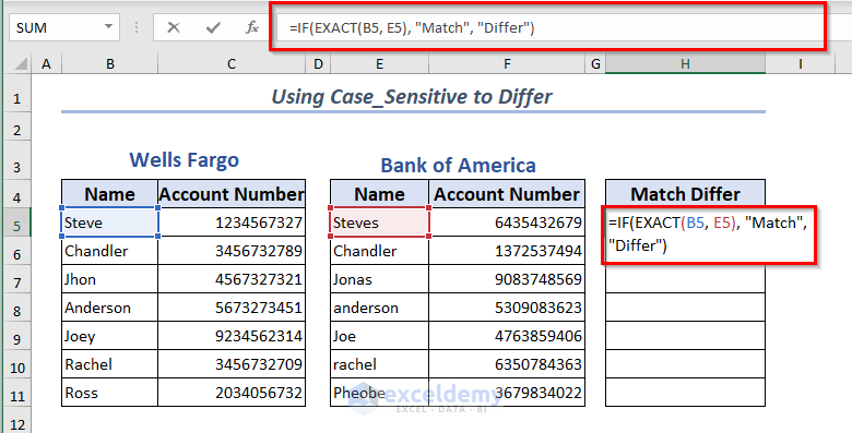
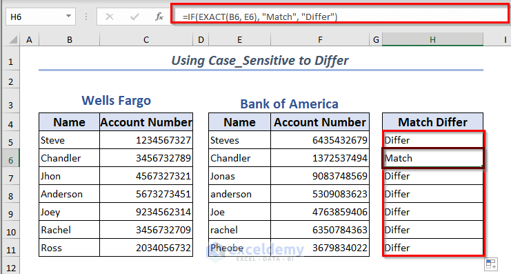
Method 5 – Matching Case Sensitive Differences
- Select a cell to place different names. Here, H5.
- Enter the Formula.
=IF(EXACT(B5, E5), "Match", "Differ")
- Press, ENTER.
- You will see the different names and also the matches.
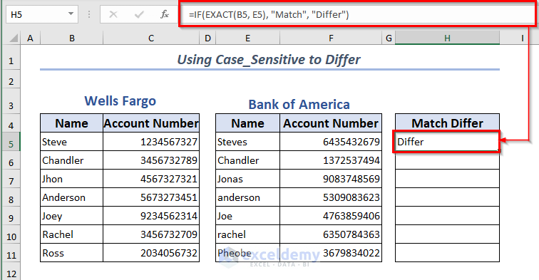
- Drag the Fill Handle to AutoFill the rest of the cells in the column.
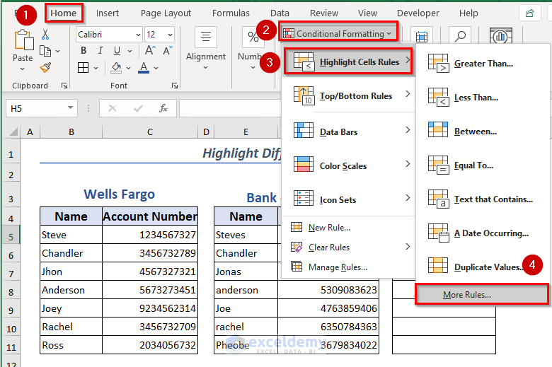
Method 6 – Highlighting Differences
- Select the cell you want to highlight for spelling differences. Here, H5.
- Go to the Home tab >> Conditional Formatting >> Highlight Cells Rule >> More Rules.
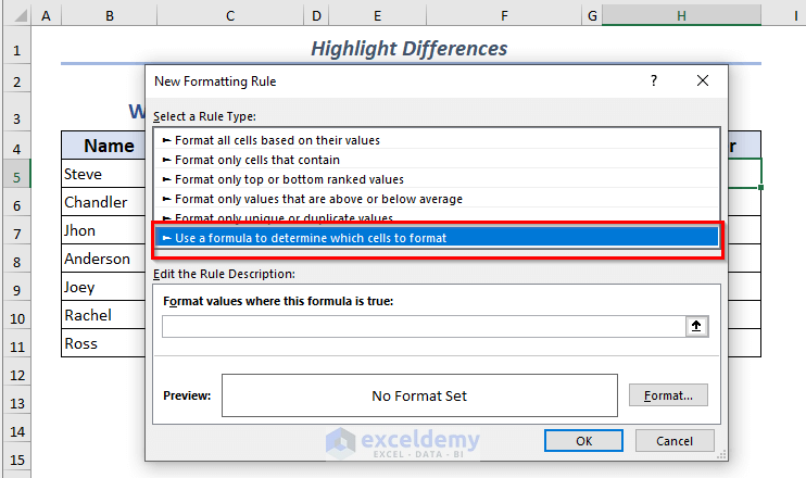
- In the dialog box, select Use a formula to determine which cell to format.
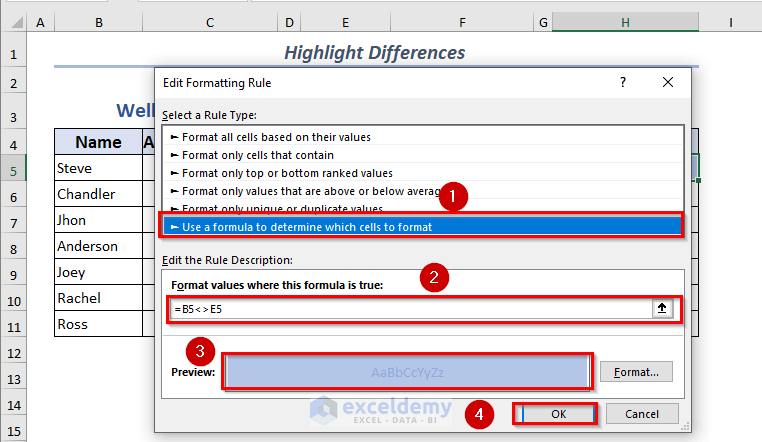
- Enter the formula =B5<>E5.
- Set the Format.
- Click OK.
- The chosen Format for different names will be displayed.
- Drag the Fill Handle to AutoFill the rest of the cells in the column.
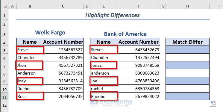
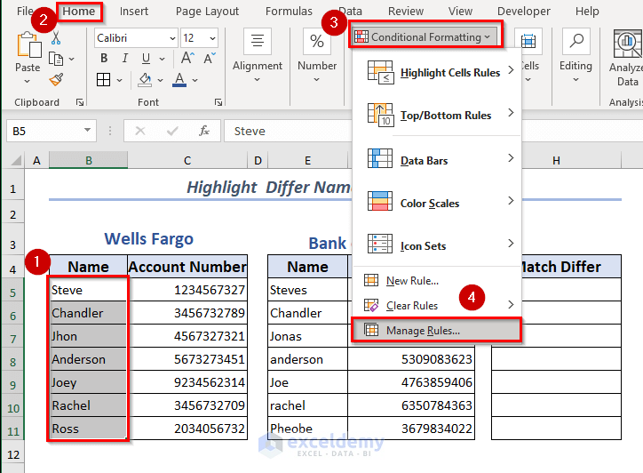
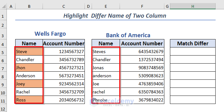
Method 7 – Matching Differences in Two Columns
- Select the cells you want to Highlight.
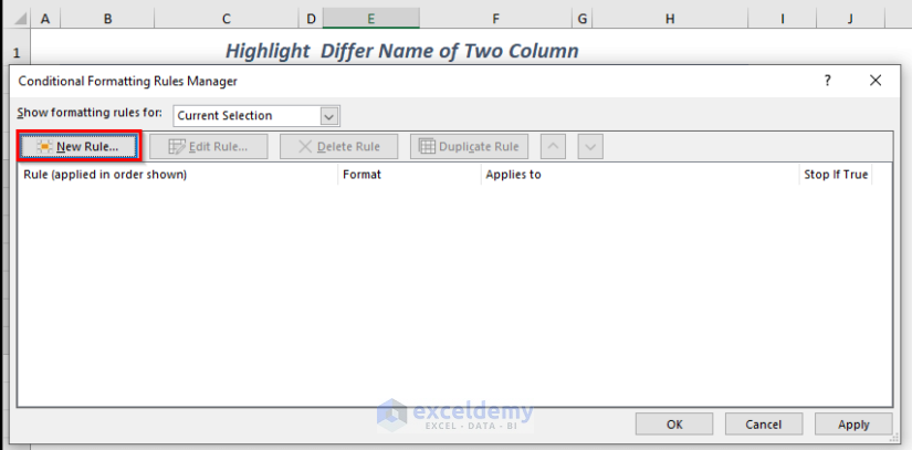
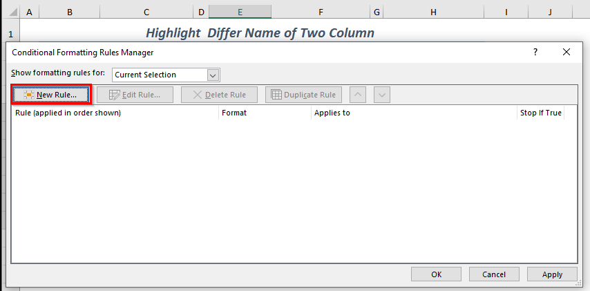
- In the Home tab >> Go to Conditional Formatting >> select Manage Rules.
- In the dialog box, select New Rule .
- Click OK.
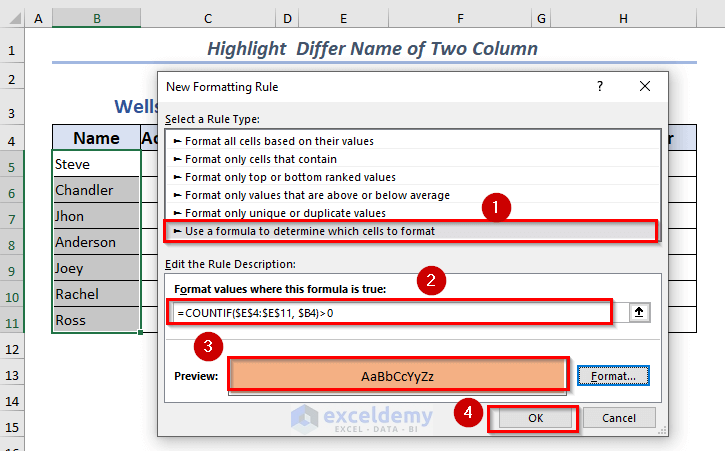
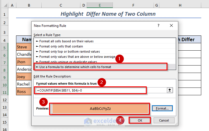
- In the new dialog box, select Use a formula to determine which cell to format.
- Enter the formula
=COUNTIF($E$4:$E$11, $B4)>0
- Set the Format.
- Click OK.
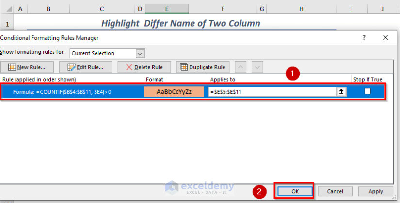
- In the new dialog box, select the formula and click OK.
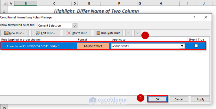
This is the output.
To apply it to Column E:
- In the Home tab >> Go to Conditional Formatting >> select Manage Rules.
- In the dialog box, select New Rule and click OK.
In the new dialog box, select Use a formula to determine which cell to format.
- Enter the formula
=COUNTIF($B$4:$B$11, $E4)>0
- Set the Format.
- Click OK.
- In the new dialog box, select the formula and click OK.
This is the output.
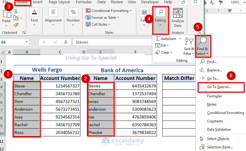
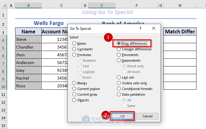
Method 8 – Using Go To Special
- In the Home tab >> Go to Find & Select >> select Go To Special.
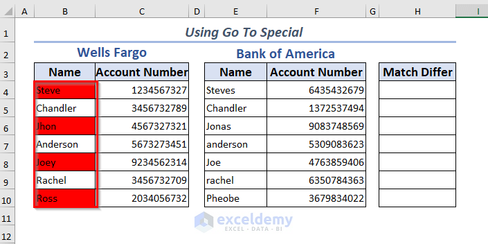
In the dialog box, select Row Differences.
- Click OK.
This is the output.
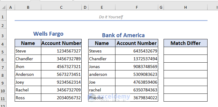
Practice Section
Download the workbook to practice.
Download Workbook to Practice
<< Go Back to | Excel Match | Learn Excel
Get FREE Advanced Excel Exercises with Solutions!

