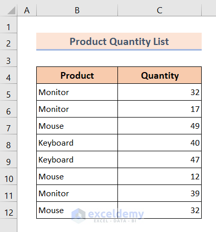
This is a sample dataset with a list of products and their quantity.
Method 1- Applying the LOOKUP Function to Pull the Last Match in Excel
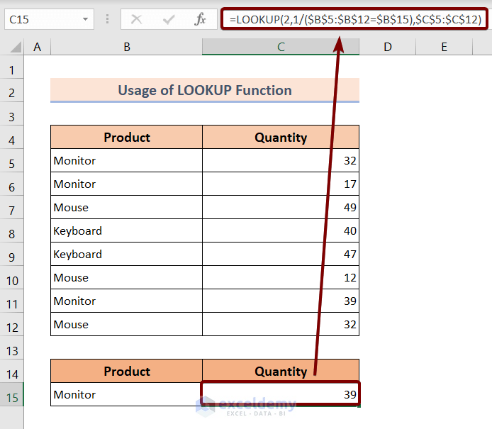
- Select C15 to store the last matched result.
- Enter the formula within the cell.
=LOOKUP(2,1/($B$5:$B$12=$B$15),$C$5:$C$12)
- Press ENTER.
Formula Breakdown
- $B$5:$B$12 is the range of cells where to look for the item, Monitor.
- $B$15 is the cell address where the lookup value is stored.
- $C$5:$C$12 is the range of cells from where the match result is returned.
- =LOOKUP(2,1/($B$5:$B$12=$B$15),$C$5:$C$12) pulls the last matched quantity for the item, Monitor.
Method 2 – Utilizing the INDEX and MATCH Functions to Return the Last Match in Excel
- Select C15 to store the last match.
- Enter the formula within the cell.
=INDEX(C5:C12,MATCH(2,1/(B5:B12=B15),1))
- Press ENTER.
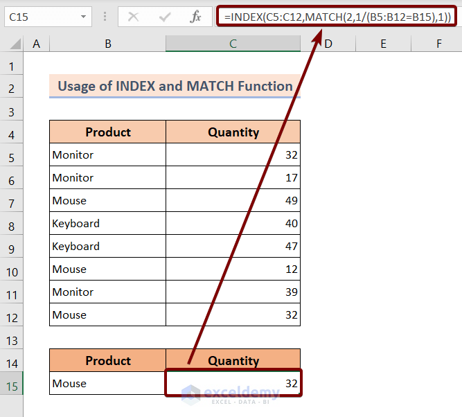
The Mouse quantity (32) is the last occurrence for this item.
Formula Breakdown
- B5:B12 is the range of cells where to search for the items.
- B15 is the cell address that holds the lookup value.
- MATCH(2,1/(B5:B12=B15),1) searches for the last occurrence of the item Mouse, and returns a numerical value, 8.
- =INDEX(C5:C12,MATCH(2,1/(B5:B12=B15),1)) looks for the quantity in the 8th row (returned by the MATCH function).
Method 3 – Using the VLOOKUP Function to Get the Last Match in Excel
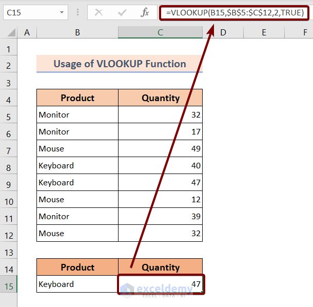
- Select C15 to store the last matched result.
- Enter the formula within the cell.
=VLOOKUP(B15,$B$5:$C$12,2,TRUE)
- Press ENTER.
Formula Breakdown
- B15 holds the lookup value – Keyboard.
- $B$5:$C$12 is the table range.
- 2 represents the column index number.
- =VLOOKUP(B15,$B$5:$C$12,2,TRUE) returns the quantity of the Keyboard item in its last occurrence.
Method 4 – Using a VBA Code to get the Last Match in Excel
- Press ALT + F11 to open up the VBA editor.
- Go to Insert ▶ Module to create a new module.
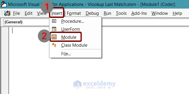
- Copy the following VBA code:
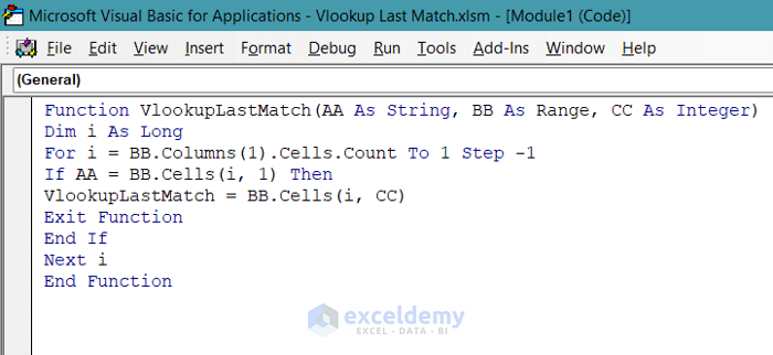
Function VlookupLastMatch(AA As String, BB As Range, CC As Integer)

Dim i As Long

For i = BB.Columns(1).Cells.Count To 1 Step -1

If AA = BB.Cells(i, 1) Then

VlookupLastMatch = BB.Cells(i, CC)

Exit Function

End If

Next i

End Function- Enter the code in the VBA editor and save it (CTRL + S can also be used to save the code).
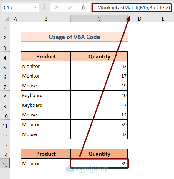
In your Excel worksheet:
- Select C15 to store the last match.
- Enter the formula within the cell.
=VlookupLastMatch(B15,B5:C12,2)
- Press ENTER.
Formula Breakdown
- B15 is cell address that contains the lookup value.
- B5:C12 is the table range.
- 2 is the column index number to return the last match.
- =VlookupLastMatch(B15,B5:C12,2) returns the quantity of the last match, Monitor.
Download the Practice Workbook
Download the Excel file and practice.
<< Go Back to | Excel Match | Learn Excel
Get FREE Advanced Excel Exercises with Solutions!

It is a very good Excel website with all the basic and advance level details .Thank you so much .
Thanks for your feedback.
Hello, is there a way to have it return a different value if the lookup value cannot be found. For example, if the product equal stand, how can I make it return “Null”?
Hi Sam
I believe you should try xlookup function it is much more flexible than vlookup.
And yes it gives you the option o f value in case that it can’t find a match
Regards
Konstantinos
Hi SAM,
The first formula: =LOOKUP(2,1/($B$5:$B$12=$B$15),$C$5:$C$12) returns #N/A error for a lookup value that cannot be found. Thus, you can add the IFERROR function to tackle this issue.
For example use the following formula to return “Null” instead of #N/A error: =IFERROR(LOOKUP(2,1/($B$5:$B$12=$B$15),$C$5:$C$12),”Null”)
I hope this is what you were looking for.
Regards!