How to Return Row Number of a Cell Match in Excel (7 Methods)

If you’re working with huge datasets and extensive search functions, you might need to locate a specific row to find additional information for a given object. You can do that by finding a row number of a cell match, which extracts the row number of a cell that contains specific text or value. Here are the most common ways to implement this type of search in your worksheets.

How to Return Row Number of a Cell Match in Excel: 7 Methods

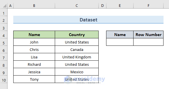
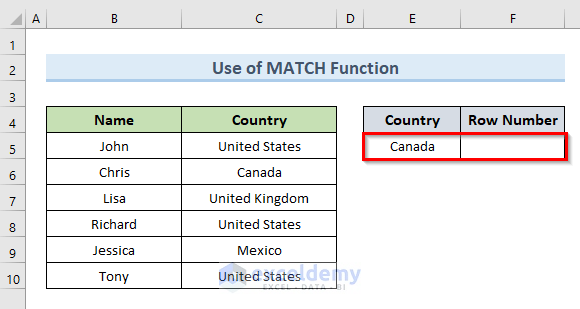
To describe the differences in the lookup process, let’s use a practice dataset for most of the methods of this article except method number 5. The dataset consists of different people’s names and their native countries. The lookup functions will search for one value either from the Name column or the Country column then determine in which row that particular value lies.

1. Return Row Number of a Cell Matching Excel with ROW Function

The simplest way to return a row number is through the ROW function. Unfortunately, unless you’re well-versed in referential functions, you’ll get limited use from it. Here’s a brute-force method you can use.

STEPS:

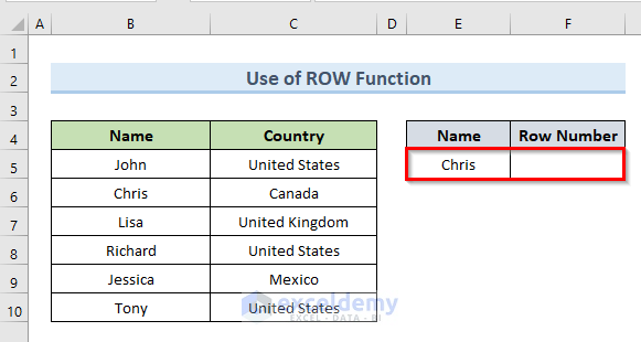
• Select cell F5.
• Write down the =ROW( part in the formula bar of that cell.
• Select the cell that contains the name Chris from the sample dataset (in columns B and C). You’ll likely get the following formula in the formula bar:

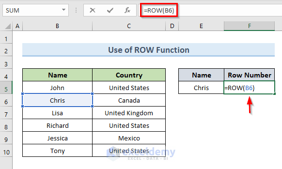
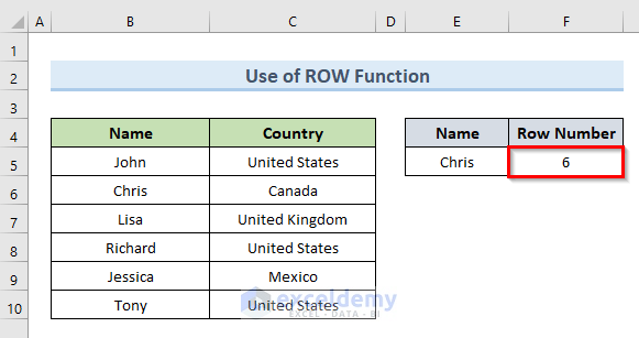
• Press Enter to confirm the cell function formatting.
• You can see the row number of the name Chris in cell F5.

2. Use MATCH Function to Get Row Number in Excel

For a more advanced method, you can use the MATCH function to return the row number of matches in Excel. The MATCH function searches a range of cells for a specified item and then returns the item’s relative location in the range. Here’s how you can use it to determine the row where the Country name Canada lies.

STEPS:

• Select cell F5.
• Insert the following formula in that cell:

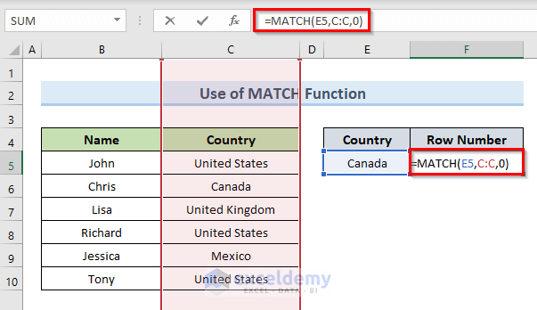
• Hit Enter.
• Behold the result!

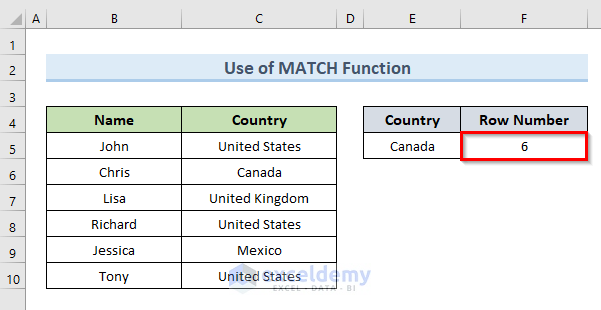
As you might’ve noticed, you have to specify the exact column to search for the value of the listed cell, meaning you have to have at least some knowledge of the table’s structure.

3. Combinations of MATCH & ROW Functions to Extract Row Sequence

Similarly to the second method, you can combine the MATCH and ROW functions to return the row number of a cell match. Same as before, the cell F5 will be the result of row number in which the value Canada lies in the Country column.

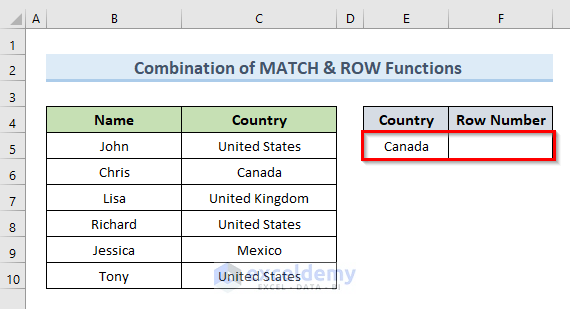
STEPS:

• Select cell F5.
• Paste the following formula in that cell:

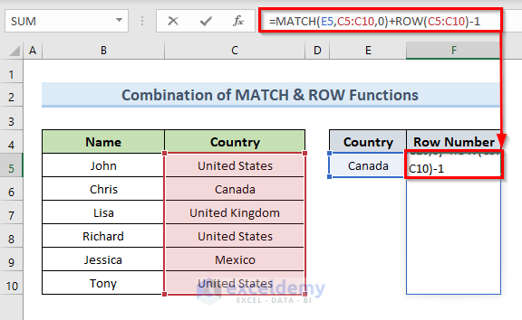
• Hit Enter.
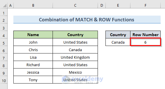
• You’ll get that the row number of the value Canada is 6 in our dataset.

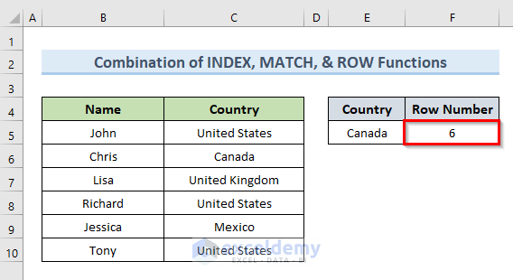
4. Combine INDEX, MATCH & ROW Functions to Return Row Number of a Match in Excel

A combination of INDEX, MATCH & ROW functions is another way to return the row number of a match in Excel.

The INDEX function returns the value at a certain point in a range or array, but it also returns a reference, making it one of the few possible arguments for a ROW function.

Let’s use the tried-and-true test of finding Canada in column C and putting its row in cell F5.

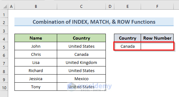
STEPS:

• In the beginning, select cell F5.
• Next, insert the following formula in that cell:

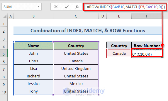
• Then, hit Enter.
• So, the above actions return the row number of the country name Canada in cell F5.

How Does the Formula Work?

• MATCH(E5,C4:C10,0): This part searches for the value of cell E5 within the range (C4:C10) and returns its relative location (2).
• INDEX(B4:B10,MATCH(E5,C4:C10,0): This part returns the reference of the matched value within the range (B4:B10) > B6.
• ROW(INDEX(B4:B10,MATCH(E5,C4:C10,0))): Returns the row number of the INDEX result > ROW(B6)=6.

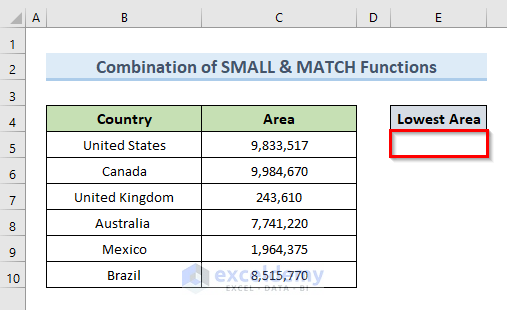
5. Merge SMALL & MATCH Functions to Get Row Number of Matched Value

We can also use the combination of SMALL & MATCH functions to return the row number of a matched value in Excel. The SMALL function returns the smallest value in a numeric list if you put 1 as its second argument. The list doesn’t have to be ordered.

To illustrate this method, you’ll need a slightly different dataset since the SMALL function only deals with numeric values. Let’s list some countries and their land areas, then find the row of the county with the smallest area in cell E5.

STEPS:

• Select cell E5.
• Type the following formula in that cell:

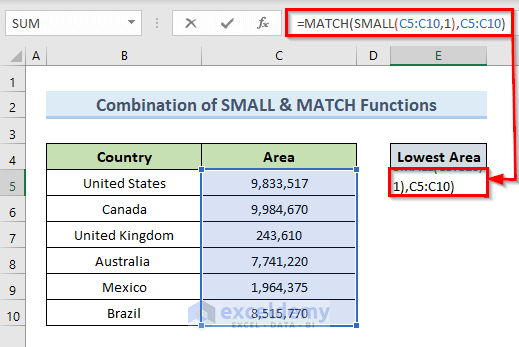
• Press Enter.
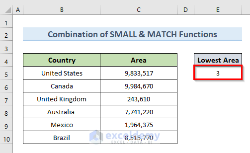
• In the end, we can see that the lowest value of the area in Column C is located in row number 3.

How Does the Formula Work?

• SMALL(C5:C10,1): This part returns the smallest numeric value from the range (C5:C10).
• MATCH(SMALL(C5:C10,1),C5:C10): Returns the row number of the smallest value in cell E5.

NOTE:

Since the MATCH function returns the relative position of a value from a data range, the above process returns the value 3 instead of 7. You can fix this by changing the second argument from C5:C10 to C:C. This forces the Match function to search through the entire row for the value indicated by the result. This might not work if your table is preceded by another table that happens to have the same value. In this case, you can append “+ROW(C4)” (put the cell reference by clicking on the table’s column header).

6. Return All Row Numbers of a Cell Match in One Cell in Excel

The methods above only work if you have one matching value throughout the column and won’t return duplicate results. If you want to list the rows for all matches, you’ll need a combination of the TEXTJOIN, IF, and ROW functions.

The TEXTJOIN function joins text from various ranges and/or strings with a delimiter of your choice (as an argument).

In the following dataset, we can see that in Column C the value of the United States is present 3 times.

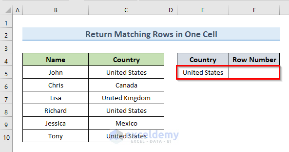
Let’s see the steps to return the row numbers having the same value in a single cell.

STEPS:

• Select cell F5.
• Input the following formula in that cell:

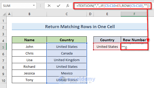
• Hit Enter.
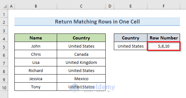
• You can see the list of row values from column C that match the cell E5.

How Does the Formula Work?

• IF(C5:C10=E5,ROW(C5:C10),””): In this part the IF formula checks which values in the range (C5:C10) are equal to the value of cell E5. After that, it returns the row number of that cell.
• TEXTJOIN(“,”,,IF(C5:C10=E5,ROW(C5:C10),””)): Combines the row numbers of the previous step with a comma in a single cell F5.

The best part about this formula is that, despite its simplicity, you can easily modify to get useful results throughout the table. If you replace the range C5:C10 both times with the entire range of the dataset (such as B4:C10), the formula will work throughout rows and columns. This essentially takes out the guesswork from finding the exact column to search.

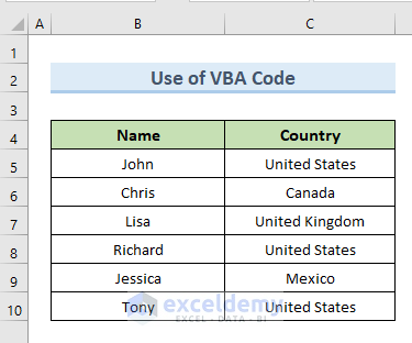
7. Apply VBA Code to Get Row Sequence of a Cell Match

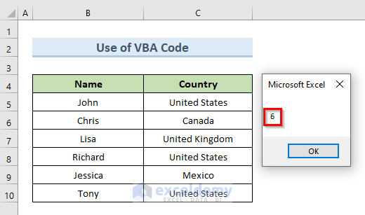
If you are an advanced Excel user, you can use VBA (Visual Basic for Applications) code to return the row number of a cell match in excel. Here’s a sample VBA code use to find out the row number of the value Canada in Column C.

STEPS:

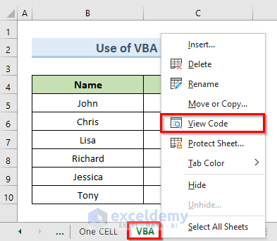
• Right-click on the active sheet named VBA in the practice workbook.
• Select the option View Code.

• A blank VBA module will appear.
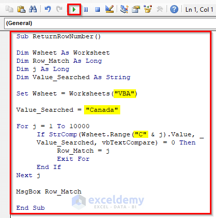
• Insert the following code in that blank module:

Sub ReturnRowNumber()
Dim Wsheet As Worksheet
Dim Row_Match As Long
Dim j As Long
Dim Value_Searched As String
Set Wsheet = Worksheets("VBA")
Value_Searched = "Canada"
For j = 1 To 10000
If StrComp(Wsheet.Range("C" & j).Value, Value_Searched, vbTextCompare) = 0 Then
Row_Match = j
Exit For
End If
Next j
MsgBox Row_Match
End Sub

• Click on the Run button or press the F5 key to run the code.

• You’ll get a message box showing that the row number of the value Canada in column C is 6.

NOTE:

If you want to search for different data from your dataset, you will just have to modify the highlighted parts of the code (see the code image above):

• Instead of “VBA” use the name of your worksheet.
• Change the value “Canada” to another value that you want to search in your worksheet.
• Instead of column range C, you need to input the column in which you want to search.

Download Practice Workbook

You can download the practice workbook from here.

Conclusion

Searching for a specific match in the entire table is a bit trickier. Out of all these methods, the sixth is probably the easiest to implement so it works regardless of what you’re trying to search. However, its results might be inaccurate if you have overlapping data points and repetitive data.

<< Go Back to | Excel Match | Learn Excel