In this article, we are going to demonstrate various examples of using the MATCH function in Excel based on different criteria, and what to do when this function doesn’t work.
Introduction to MATCH Function in Excel
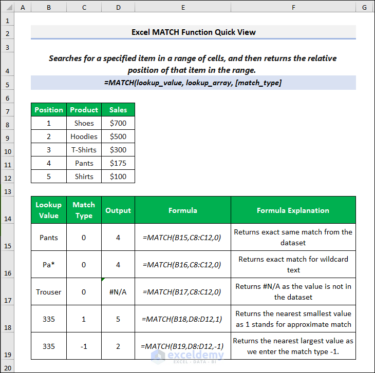
The MATCH function in Excel is used to locate the position of a lookup value in a row, column, or table, and returns the relative position of an item in an array that matches a specified value in a specified order.
- Syntax:
=MATCH(lookup_value,lookup_array,[match_type])
- Arguments Explanation:
| Argument | Required/Optional | Explanation |
|---|---|---|
| lookup_value | Required | The value to match in the array |
| lookup_array | Required | A range of cells or an array reference in which to lookup the value |
| match_type | Optional | Specifies how Excel matches lookup_value with values in the lookup_array. 1 = exact or next smallest, 0 = exact match and -1 = exact or next largest |
- Return Value:
Returns the lookup value’s relative position.
- Available Version:
From Excel 2003 onwards.
How to Use MATCH Function in Excel: 8 Practical Examples
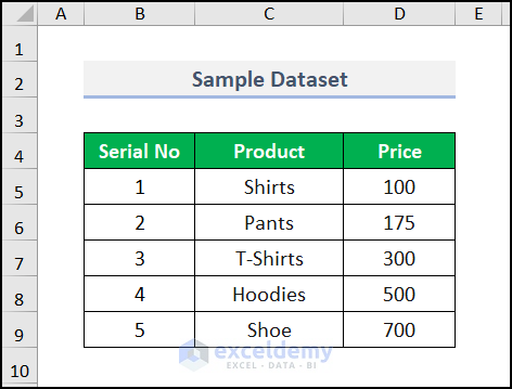
To demonstrate the uses of the Match function, we’ll use the following dataset containing some “Products” with their ‘Price” and ‘Serial Numbers” to find out the exact or approximate match for our search value.
We used the Microsoft 365 version of Excel here, but the methods should work in any other version from Excel 2003 onwards.
Example 1 – Finding the Position of a Value
1.1 – Exact Match
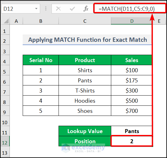
For an exact match, simply set the matching_criteria argument to 0.
Steps:
- In cell C12, enter the following formula.
The lookup_value is cell D11, the lookup_array is C5:C9, and the matching_criteria is 0 for an exact same match. So this MATCH function returns the position in the lookup_array of the exact value in cell D11.
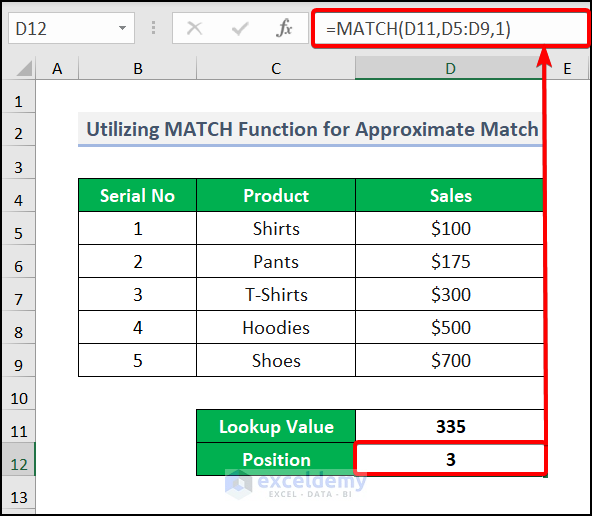
1.2 – Approximate Match
In most cases, rather than an exact match, an approximate match is used for numbers.
Steps:
- Insert the below formula in cell D12:
Here, the D5:D9 cell range is the lookup_array. Since an approximate match is our target, we set 1 in the match_type field, which returns the nearest smallest value to the lookup_value. 300 is the nearest value to 335, so our formula returned the position of 3.
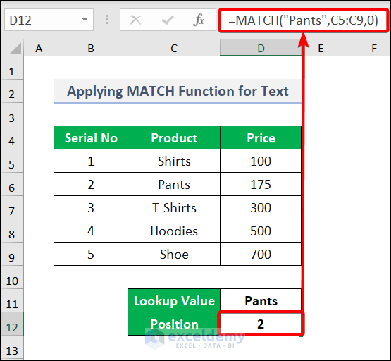
1.3 – Specific Text Match
The MATCH function can also take text as its lookup value, as opposed to the cell reference used above. This is useful if you want to find the value or position of particular text in your dataset without knowing the cell reference.
Steps:
- Enter the following formula in cell D12:
The formula takes the lookup_value “Pants” and searches for an exact match in the lookup_array C5:C9.
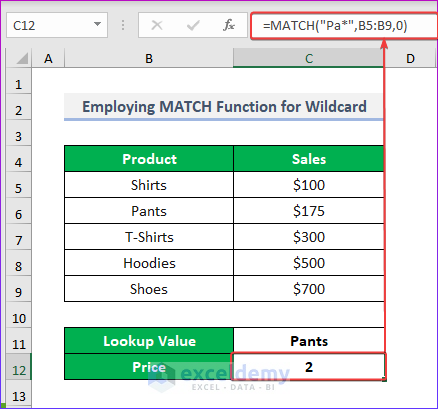
1.4 – Wildcard Match
You can also match text partially and return the position of the partial match in the dataset using a wildcard. For example, to find out the position for the product “Pants“, we can use the wildcard ” Pa*” instead of the full text.
Steps:
- Enter the below formula in cell C12:
Here, the MATCH function finds an exact match (matching_criteria = 0) in the lookup_array of B5:B9 for the lookup_value Pa*. Then the INDEX function takes the result of the MATCH function and finds the relation between the C5:C9 array and the Pa* text.
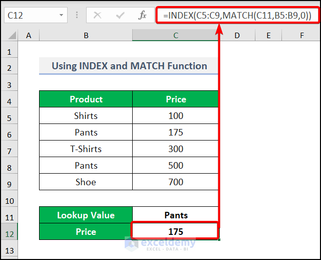
Example 2 – Finding a Value Corresponding to Another Value
We can also find a value corresponding to another value by using the INDEX function along with the MATCH function. The INDEX function returns the value at a given location in a range or array. Then the MATCH function checks for the match.
Steps:
- In cell C12 insert the following formula:
B5:B9 is the array where we need to find the value. Using the MATCH function, we set the row_number, here 2. Then, from the array B5:B9, the INDEX function returns the value in the position of row 2.
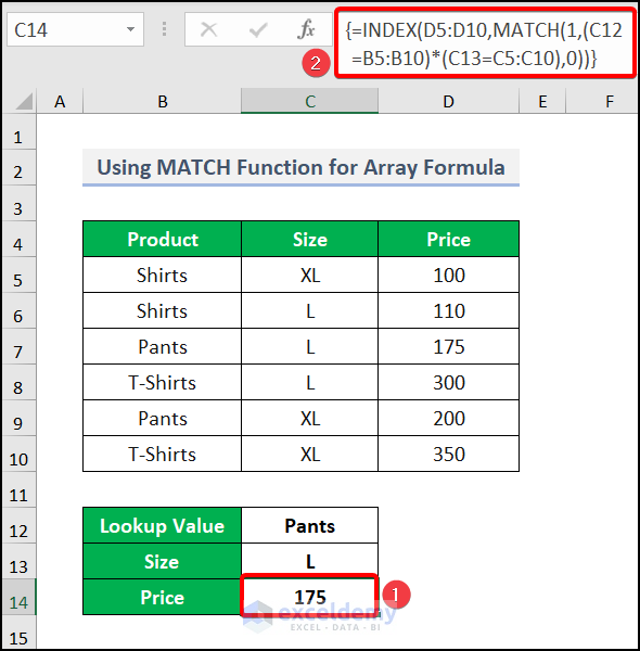
Example 3 – Applying the MATCH Function in Array Formula
We also need the INDEX function to use the MATCH function in an array formula.
Steps:
- In cell C14 enter the following formula:
Here we use 1 as the lookup_value in MATCH. The lookup_array is combined by multiplying the results from checking two criteria within their respective columns.
The (C12=B5:B10) and (C13=C5:C10) criteria provide an array of TRUE or FALSE. By multiplying the arrays, another array of TRUE and FALSE is formed. TRUE can be represented as 1, so we are looking for the position of the TRUE value inside the array.
Since this is an array formula, press CTRL + SHIFT + ENTER to execute it if you’re not a Microsoft 365 subscriber (where just pressing Enter will suffice).
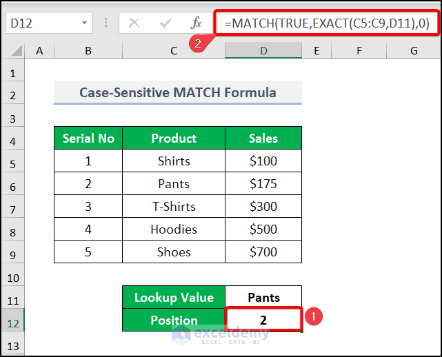
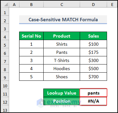
Example 4 – Utilizing Case-Sensitive MATCH Formula
For case-sensitive text, use the EXACT function and then the MATCH function to match the criteria. The structure of the formula is slightly different from that of the MATCH function formulas used in the above examples.
Steps:
- Enter the following formula in cell D12:
The EXACT(C5:C9, D11) syntax returns an exact match in the lookup_array C5:C9, and the logical argument TRUE represents the existing value from the EXACT function.
But when we use a lowercase letter in the lookup_value then it returns #N/A. So this formula works accurately, because an exact, case-sensitive match is required.
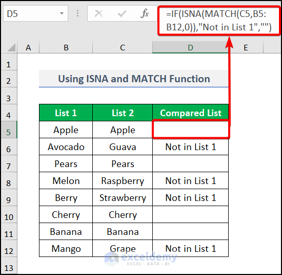
Example 5 – Comparing Two Columns Using ISNA and MATCH Functions
Suppose we have a dataset of 2 lists, and we want to compare the 2nd list with the 1st one and return the values that don’t appear in the first list. We can do this using the ISNA and MATCH functions, along with the IF function to display the logical result in text format.
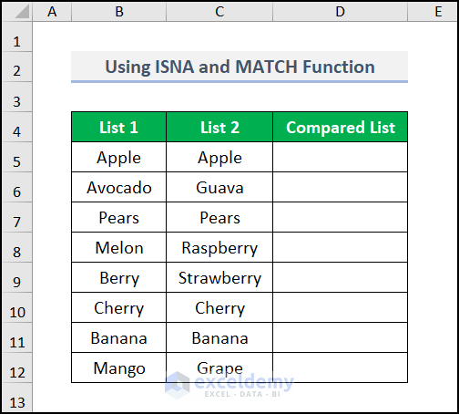
Steps:
- In cell D5 enter the following formula:
Here, the MATCH function in Excel returns TRUE for an exact match and FALSE otherwise. Then the ISNA function flips the results received from the MATCH function. Finally, the IF function returns the logical output as text.
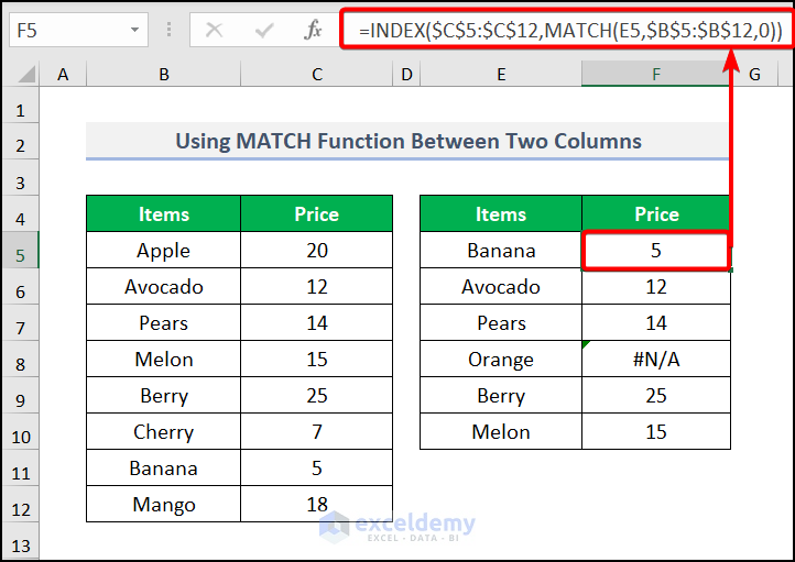
Example 6 – Applying the MATCH Function Between Two Columns
Suppose we have a list of products that match a previous column, and we want to put the value of “Price” that is an exact match in our new column. To do this, we need to use the INDEX and MATCH functions together.
Steps:
- In cell F5 enter the formula below:
This formula compares the text between columns B and E and returns the matching value.
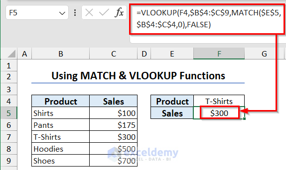
Example 7 – Use the MATCH Function with VLOOKUP in Excel
When using the VLOOKUP function to look up a value from a dataset, deleting or inserting any column from that dataset will break the function.
In that case, use the MATCH function with VLOOKUP to do the task. To look up the Sales value of a product, we can use the following formula:
=VLOOKUP(G4,$B$4:$D$9,MATCH($F$5,$B$4:$D$4,0),FALSE)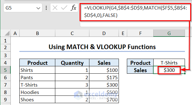
In the formula, we use the cell range B4:D9 as table_array. Now, if we delete the Quantity column, the formula will change the table_array to B4:C9 and show the result.
Example 8 – Apply HLOOKUP with the MATCH Function to Lookup Values in a Horizontal Dataset
Similarly, use the HLOOKUP function to look up values in a horizontal dataset. Use the following formula to do that:
=HLOOKUP(C8,B4:G6,MATCH(B9,B4:B6,0),FALSE)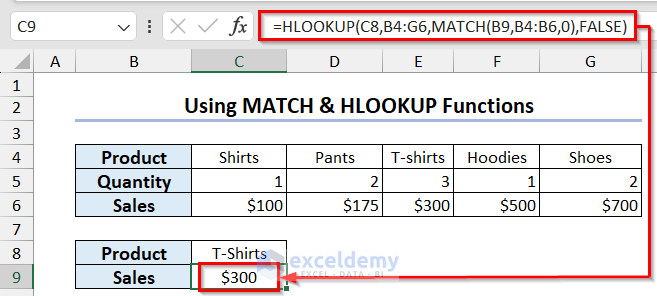
Read More: Excel MATCH Function Not Working
Frequently Asked Questions
1 – Is the MATCH function better than the VLOOKUP function?
No, the VLOOKUP function is better as it returns a value rather than the position of a value like the MATCH function. However, by combining these two functions you can look for a value from a dataset, and deleting any row or column will not change the result.
2 – What does the MATCH function return if no match is found?
The error value #N/A.
3 – Can the MATCH function work with both rows and columns?
Yes. The lookup_array can be a single row or a single column.
4 – Can the MATCH function figure out the difference between uppercase and lowercase values?
No.
Download Practice Workbook
Download the following practice workbook. It will help you to realize the topic more clearly.
<< Go Back to Excel Functions | Learn Excel
Get FREE Advanced Excel Exercises with Solutions!
