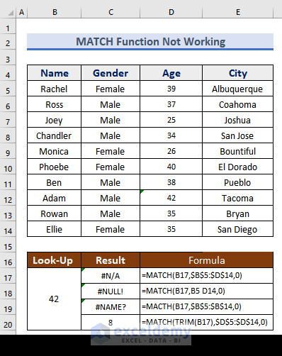
While working on a vast data set you sometimes get stuck with the MATCH function not working issue. So, to help you overcome this issue, we will cover the possible reasons in this article, that are responsible for why your Excel MATCH function is not working. In the following picture, you will find out error message associated with the MATCH function.
When MATCH Function Not Working in Excel: 3 Cases with Solutions
Case 1: #N/A! Error
#N/A Error is one of the most common errors associated with the MATCH Function. There are several reasons behind this error. This error occurs if Excel cannot find source data in the table array. If the look_up value is in text format, the MATCH function will return the #N/A error. You also get this error when you do not insert syntax properly.
However, to overcome this issue, you can follow the solutions below.

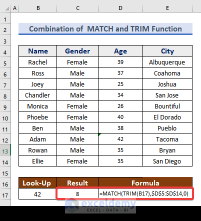
Solution 1: Combine MATCH and TRIM Functions to convert Numbers into Text
We can apply the MATCH and TRIM functions to fix the #N/A error. The MATCH function returns the #N/A error while the data of the table array is in text format. Follow the steps to overcome this issue.
Steps:
- First of all, select C17.
- Then write down the following formula as,
=MATCH(TRIM(B17),$D$5:$D$14,0)
- After that, press Enter. As a result, it should work adequately as below.
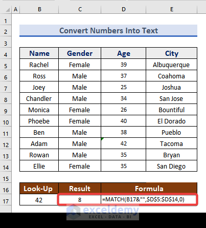
Solution 2: Convert Numeric Value to Text
You can solve the #N/A error by converting the numerical value to the text. Let’s follow the instructions below to learn!
Steps:
- To begin with, select C17.
- Afterward, insert the following formula in that cell.
=MATCH(B17&"",$D$5:$D$14,0)- Hence, press Enter Then it will erase the error and display the result as follows.
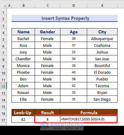
Solution 3: Insert Syntax Properly
Another solution to the problem is the insertion of syntax properly. Follow the steps below.
Steps:
- Firstly, select C17.
- Hence write down the formula as
=MATCH(B17,$D$5:$D$14,0)- When writing the formula is done, hit Enter The outcome looks like this below
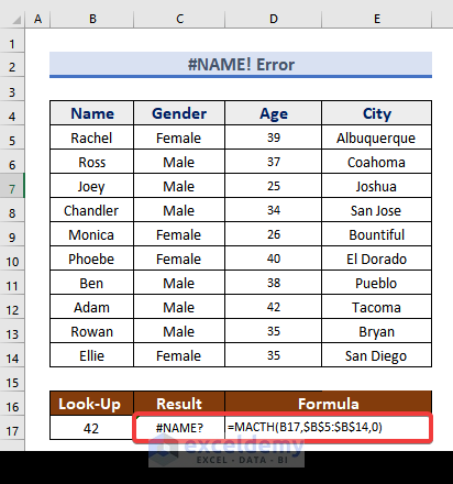
Case 2: #NAME! Error
Excel shows the #NAME error if a non-existent function is used. It happens especially when the user misspells the function’s name and it shows this error. Let’s look at the picture attached below, it shows the #NAME error because the MATCH Function is typed as MACTH.
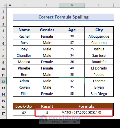
Solution: Correct Formula Spelling
To solve this #NAME error issue, follow the instructions properly.
Steps:
- In the beginning, select
- Subsequently, write down the formula as
=MATCH(B17,$D$5:$D$14,0)- Later, press Enter Eventually, this error should be gone.
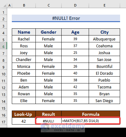
Case 3: #NULL! Error
The #NULL! error message appears when unexpected space is added or if the Colon in the range is omitted.
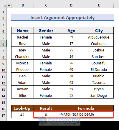
Solution: Insert Argument Appropriately
Inserting the correct formula with the appropriate argument can resolve the issue. Follow the steps below.
Steps:
- First of all, select C17.
- Afterward, write down the formula as
=MATCH(B17,$D$5:$D$14,0)- Hence, press Enter And it should remove the Error message.
Read More: Excel MATCH Function Match Type
Download Practice Workbook
Download this practice workbook to exercise while you are reading this article.
Conclusion
This article covered the main reasons why the MATCH Function in your Excel is not working. Additionally, you can practice this Excel problem by downloading from this page. Yet, if you have any queries related to this problem please comment below.
<< Go Back to Excel MATCH Function | Excel Functions | Learn Excel
Get FREE Advanced Excel Exercises with Solutions!
