Introduction to the Excel TRIM Function
The Excel TRIM function is categorized under the TEXT functions. It removes the extra spaces from a text string.
Objectives
Remove all spaces from a text string except for single spaces between words.
Syntax

=TRIM (text)Arguments Explanation
| Argument | Required/Optional | Explanation |
|---|---|---|
| text | Required | The text string from which to eradicate unnecessary spaces |
Version
- The DVAR function is available from Microsoft Excel 2007.
- Here, we will use Microsoft Excel 365.
Method 1 – Using the TRIM Function to Remove Extra Spaces from Left/Right
Steps:
Our example dataset contains a few movie names.
- To remove these extra spaces, we need to provide the Cell Reference of the text by applying the following formula:
=TRIM(B5)- Select B5 as the Cell Reference for the first row of the Movie
- Press Enter.
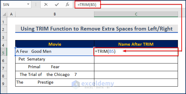
You can see the spaces between Few and Good have been eradicated (only one space remains).
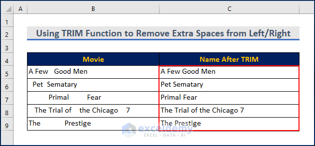
- Use the Fill Handle tool and drag it down from cell C5 to cell C9.
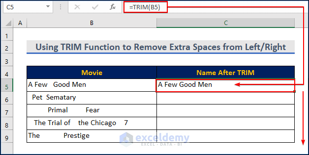
- A similar formula (change in Cell Reference) will remove the spaces from the beginning, middle, and end for the rest of the rows.
Method 2: Combining TRIM and CLEAN Functions to Remove Spaces and Clean String
Steps:
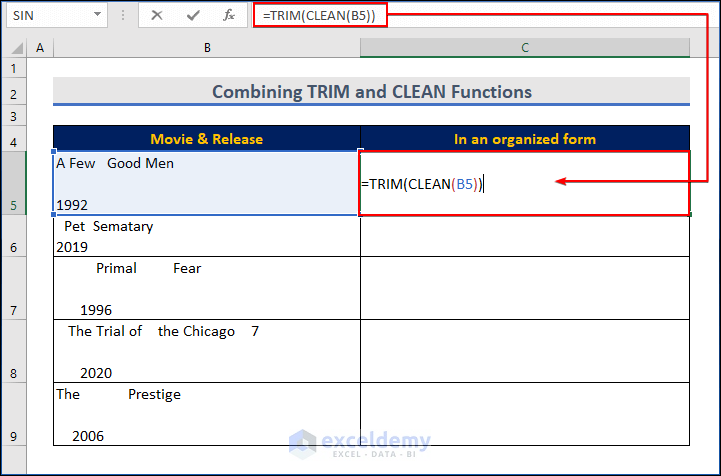
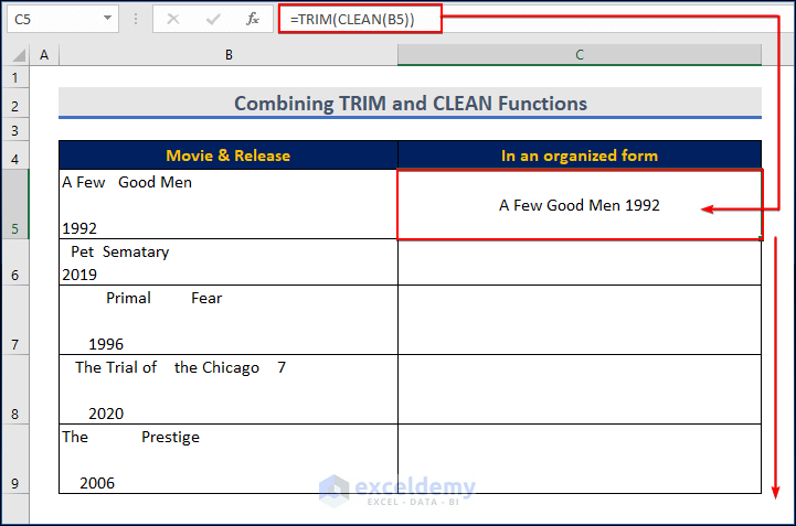
- We have brought the dataset of movie names and their respective release years here. Movie names and the release year are in different lines.
- There are also extra spaces. To eradicate the issues and organize the data, we are going to use a function called CLEAN along with the TRIM function.
- The CLEAN function converts text to be cleaned of line breaks and other non-printable characters.
- For the first row, our formula will be
=TRIM(CLEAN(B5))- Press Enter.
- You can see the spaces between the texts in cell C5 in an organized form.
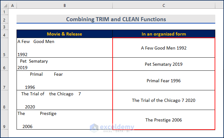
- Use the Fill Handle tool and drag it down from cell C5 to cell C9.
- The formula provided the cleaned data, no extra spaces, and no line breaks.
Read More: How to Trim Spaces in Excel
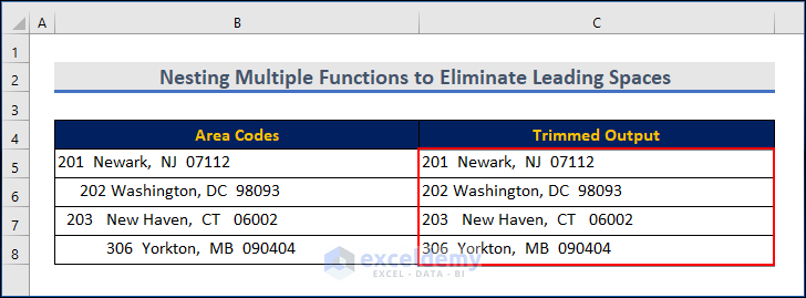
Method 3 – Nesting Multiple Functions with TRIM to Eliminate Leading Spaces
Steps:
- The area codes have spaces at the beginning as well as in between the words. We aim to remove the spaces from the beginning only.
- We will use MID, FIND, and LEN functions. To learn more about these functions, visit the following articles: MID, FIND, LEN.
- The formula will be:
=MID(B5,FIND(MID(TRIM(B5),1,1),B5),LEN(B5))- Press Enter.
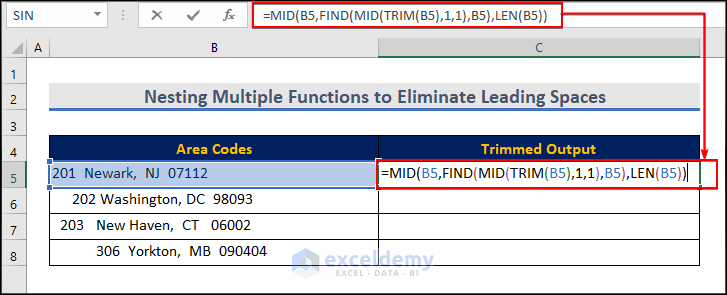
- The combination of FIND, MID, and TRIM calculates the position of the first text character in a string.
- Supply that number to the outer MID function so that it returns the entire text string starting at the position of the first text character.
- You can see that there are no leading spaces available in the given image.
- Use the Fill Handle tool and drag it down from cell C5 to cell C9.
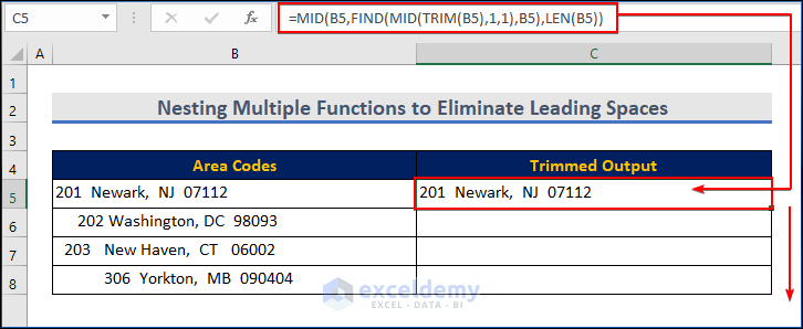
- You will get the final output in the image below.
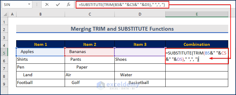
Method 4 – Merging TRIM and SUBSTITUTE Functions to Remove Spaces with Concatenation
Steps:
- Choose cell E5.
- Enter the following formula:
=SUBSTITUTE(TRIM(B5&" "&C5&" "&D5)," ",", ")- Press Enter.
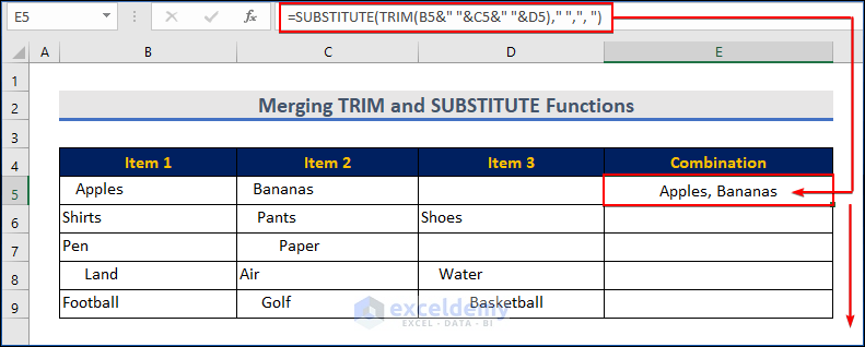
- TRIM effectively removes all white space from the beginning and end of a string while leaving only one space between each word. It handles additional space brought on by blank spaces.
The SUBSTITUTE can be used to replace the space between two elements. So, each space (” “) is changed to a comma and space using the SUBSTITUTE command (“, “).
- You will see here that this formula can concatenate the values in the below image.
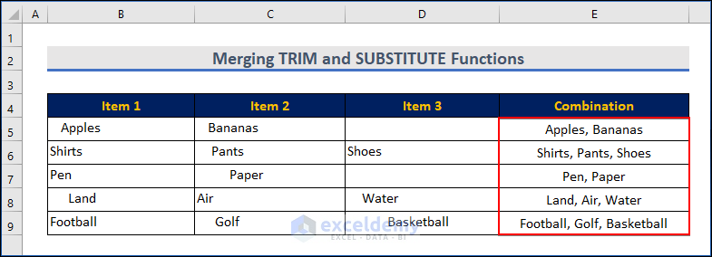
- Use the Fill Handle tool and drag it down from cell E5 to cell E9.
You will find all the texts have been concatenated with the removal of extra spaces.
Method 5: Combining LEN and TRIM Functions to Count and Highlight Extra Spaces
Steps:
- Select cell C5.
- To find the extra spaces in the string, enter the following formula:
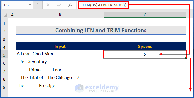
=LEN(B5)-LEN(TRIM(B5)) - Press Enter.
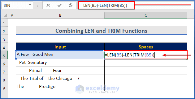
- LEN function provides the length of the string. To learn more about the function, visit the LEN.
- LEN(B5) provided the full length of the string of cell B5 and LEN(TRIM(B5)) provided the length after trimming. And the subtraction of these two will provide the total number of extra spaces.
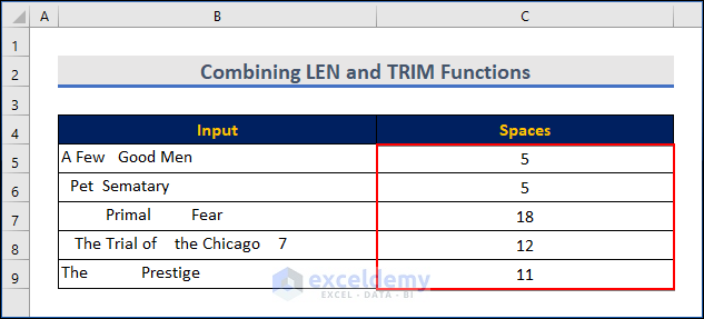
- You will see here that this formula can count the spaces in the image below.
- Use the Fill Handle tool and drag it down from cell C5 to cell C9.
You will get all the results.
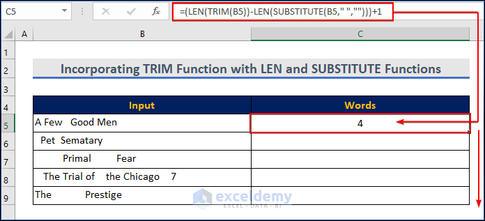
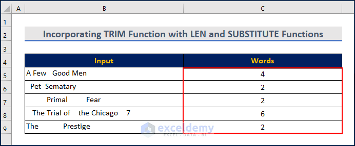
Method 6 – Incorporating the TRIM Function with LEN and SUBSTITUTE Functions for Counting Words
Steps:
- Use the LEN and SUBSTITUTE functions along with TRIM.
- Choose cell C5.
- Enter the following formula:
=(LEN(TRIM(B5))-LEN(SUBSTITUTE(B5," ","")))+1- Press Enter.

- The SUBSTITUTE function removes all spaces from the string, and then LEN calculates the length without spaces.
- This number is then subtracted from the length of the text with spaces. We have used TRIM to eradicate any spaces at the beginning or end of the string.
- Finally, 1 is added to the result since the number of words is the number of spaces + 1.
- You will find the number of words from this string.
- The same formula will provide the number of words for the rest of the texts by using the Fill Handle tool.
As a result, we have found the number of words from this string for all the cells.
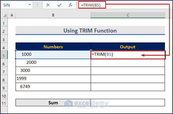
Example 7 – Combining TRIM and VALUE Functions to Delete Spaces for Numerical Values
Steps:
- Choose cell C5.
- Apply the trim function below:
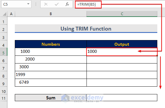
=TRIM(B5)- Press Enter.
- You can see the first trimmed number here.
- Use the Fill Handle tool and drag it down from cell C5 to cell C9.
- We have found the trimmed number.
- But are they really numbers? Let’s check by summing them together.
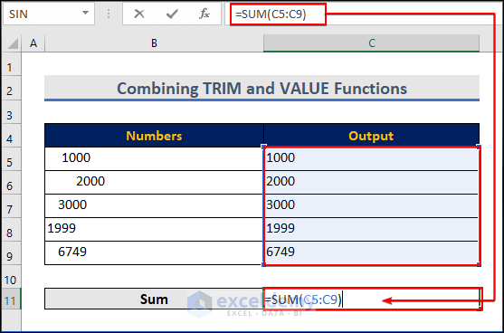
- Choose cell C11 and enter the following formula:
=SUM(C5:C9)- Press Enter.
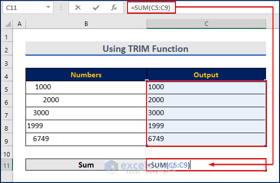
- The sum of the values is 0.
- This is because the digits you see are not numbers. They are in the Text format.

- To convert these into numbers after TRIM, we will use a function
- The formula will be
=VALUE(TRIM(B5)) - Press Enter.
- The first-row value became So, for the rest of the values, we are using the AutoFill feature.
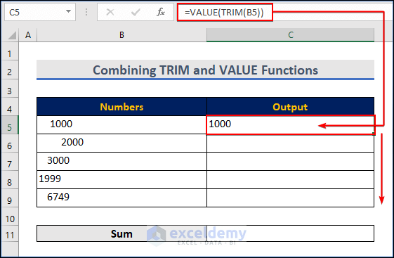
- Therefore, you can see all the output in the number format
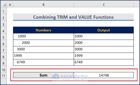
- All the values are now Numbers, and they can be added.
The image shows the sum of all the numbers.
Download the Practice Workbook
Download the following Excel workbook to practice.
Excel TRIM Function: Knowledge Hub
- How to Trim Part of Text in Excel
- How to Trim Right Characters and Spaces in Excel
- How to Use Left Trim Function in Excel
- [Fix] TRIM Function Not Working in Excel
<< Go Back to Excel Functions | Learn Excel
Get FREE Advanced Excel Exercises with Solutions!
