How to Use FIND Function in Excel (7 Suitable Examples)

In Microsoft Excel, the FIND function is generally used to extract the position of a defined text in a cell containing a text string. In this article, you’ll get to learn how you can use this FIND function effectively in Excel with appropriate illustrations.

The above screenshot is an overview of the article, representing a few applications of the FIND function in Excel. You’ll learn more about the methods along with the other functions to use the FIND function precisely in the following sections of this article.

Introduction to the FIND Function

• Function Objective:

FIND function returns the starting position of a case-sensitive text string within another text string.

• Syntax:

=FIND(find_text, within_text, [start_num])

• Arguments Explanation:

• Return Parameter:

A numerical value in an integer form that defines the position of the defined character in a text string.

How to Use FIND Function in Excel: 7 Suitable Examples

1. Using FIND Function to Extract the Position of a Specified Character in a Text

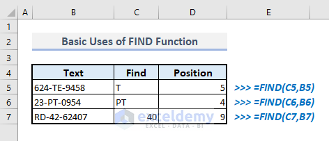
In the following picture, Column B contains a few text values and Column C represents what is to be found in the texts in Column B. In Column D, we’ll extract the positions of the characters defined in Column C.

In Cell D5, the formula with the FIND function will be:

After pressing Enter, the function will return 5 which means the letter ‘T’ lies in the 5th position in the text in Cell B5. Similarly, you can find the next two outputs in Cells D6 and D7.

2. Use of FIND Function for Case-Sensitive Character(s) in Excel

While using the FIND function, you have to keep in mind that this function is responsible for extracting case-sensitive text from a cell. If the FIND function cannot find a text in a string with a case-sensitive match, then it’ll return a #VALUE error.

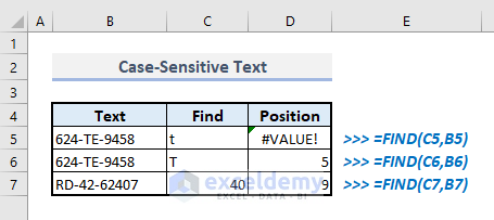
For example, in Cell D5, ‘t’ with lower-case cannot be found in Cell B5 and that’s why if you input ‘t’ as find_text argument, you’ll be shown the #VALUE error. In Cell D5, we’ve defined the find_text argument with ‘T’ and as a result, the function has returned an integer which is defining the position of ‘T’ in the text string in Cell B6.

3. Extracting Text from the Beginning of a String up to a Certain Position with FIND Function

If you have a dataset with a list of texts from which you have to extract the initial parts only then the combination of MID and FIND functions should be handy enough. The MID function returns the characters from the middle of a text string, given a starting position and length. The generic formula of this MID function is:

=MID(text, start_num, num_characters)

For example, in Column B, there are some texts with spaces inside and we have to extract the first names or words only.

In the output Cell C5, the related formula will be:

After pressing Enter, you’ll be displayed the word from the beginning of the text in Cell B5.

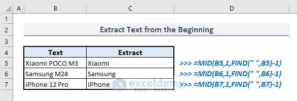
In this formula, the starting_num for the MID function is 1 which means the output text will start from the first character in Cell B5. FIND function defines the number of characters or character length up to the first space.

4. Drawing Out Text from the End of a String with FIND Function in Excel

With the combination of RIGHT, LEN and FIND functions, we can extract the text or word from the end of a text string. The RIGHT function returns the specified number of characters from the end of the text string whereas the LEN function returns the number of characters in a text string.

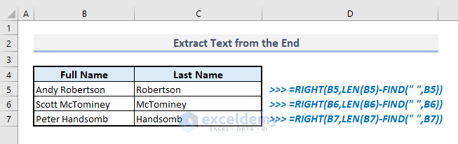
In Column B, a few names are lying and in Column C, we have to pull out the last names only. So, the related and combined formula in the output Cell C5 will be:

Press Enter and you’ll find the last name of Andy Robertson.

🔎 How Does the Formula Work?

➤ FIND function returns the position of the first space from the text in Cell B5 and that is 5.

➤ LEN function returns the total number of characters from the text string in Cell B5 and that is 14.

➤ The difference between the previous two outputs is defined as the second argument for the RIGHT function which represents the number of characters from the end of a text string.

➤ Finally, the RIGHT function extracts the last name defined by the number of characters from the end of that text string.

5. Finding the Position of a Character Multiple Times with FIND Function 

Let’s think of a range of cells where we have to find the position of a similar character multiple times in a text string. For example, from Cell B5, we’ll find out the positions of the 1st and 2nd spaces in the text string. To find the position of the first space, the related formula in Cell C5 will be:

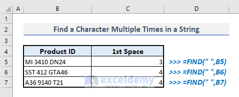
And to find the position of the second space in the text string lying in Cell B5, the related formula in the output Cell D5 will be:

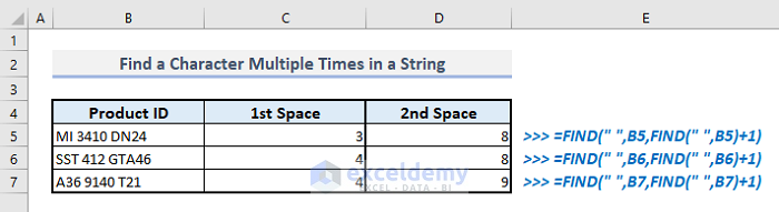
Read More: FIND Function Not Working in Excel 

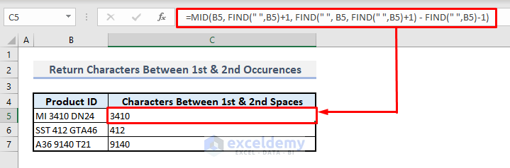
6. Returning All Characters Between the 1st & 2nd Occurrences with FIND Function

Now Column B has several texts with two spaces. We’ll extract the text between those two spaces in Column C for each case.

In the output Cell C5, the related formula will be:

After pressing Enter, the formula will return the extracted data lying between the two spaces from the text string in Cell B5.

🔎 How Does the Formula Work?

➤ In the second argument (start_num) of the MID function, the FIND function defines the starting number of the character as the position of the first space.

➤ FIND(” “, B5, FIND(” “,B5)+1) – FIND(” “,B5)-1; this part defines the number of characters before the second space from the starting position found in the previous step.

➤ Finally, the MID function returns the extracted text value based on the described arguments.

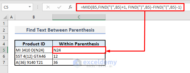
7. Pulling Out Text within Parenthesis with FIND Function in Excel

In Column B, there are a few texts with parenthesis inside. We’ll extract the data lying inside the parentheses only.

The required formula with FIND and MID function in the output Cell C5 will be:

Press Enter and you’ll get the text between parentheses at once.

🔎 How Does the Formula Work?

➤ In the second argument of the MID function, the FIND function defines the starting number for the MID function as the position of the ‘(‘ and by adding 1 to it.

➤ The third argument of the MID function, FIND(“)”,B5)-FIND(“(“,B5)-1, defines the number of characters between the opening and closing brackets.

➤ Finally, the MID function returns the extracted data or text within the parenthesis.

💡 Things to Keep in Mind

🔺 If more than one character is included in the FIND function, it’ll return the position of the first character only.

🔺 FIND function does not support wildcard characters as it extracts the position of the defined text only in a numerical value.

🔺 As the FIND function is case-sensitive, the function will be unable to find the character if you include a text with the wrong case(s) as the find_text argument, and thereby the function will return a #VALUE error.

🔺 To avoid case-sensitivity, use the SEARCH function instead of the FIND function.

🔺 If the find_text argument is empty, the function will return 1.

🔺 If the input in the find_text argument is found more than once in the selected text string, the function will return the position of the first finding only.

Download Practice Workbook

You can download the Excel workbook that we’ve used to prepare this article.

Concluding Words

I hope all of the suitable methods mentioned above to use the FIND function will now prompt you to apply them in your Excel spreadsheets with more productivity. If you have any questions or feedback, please let me know in the comment section. Or you can check out our other articles related to Excel functions on this website.

<< Go Back to Excel Functions | Learn Excel