Introduction to ISNUMBER Function
- Function Objective
The ISNUMBER function checks whether the value of a cell is a number or not.
- Syntax
=ISNUMBER(value)- Arguments Explanation
| ARGUMENT | REQUIRED/OPTIONAL | EXPLANATION |
| value | Required | Insert the value you want to check if it is a number or not. |
- Return Parameter
Returns TRUE if the value is a number, otherwise returns FALSE.
Introduction to MATCH Function
- Function Objective
The MATCH function is used to match values from a given cell range.
- Syntax
=MATCH(lookup_value, lookup_array, [match_type]- Arguments Explanation
| ARGUMENT | REQUIRED/OPTIONAL | EXPLANATION |
| lookup_value | Required | The value you want to match |
| lookup_array | Required | The cell range or an array where you want to find the value |
| match_type | Optional | Instructs how to find the match value.
Here, 1= Less than, 0= Exact match, -1= Greater than |
- Return Parameter
Returns the relative position of the lookup value.
Dataset Overview
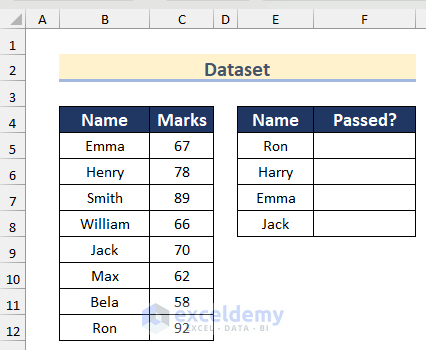
Let’s say we have a dataset containing Names and Marks of some students who wrote an exam. We want to check if certain students Passed or Failed by matching their names. Here are the two methods:
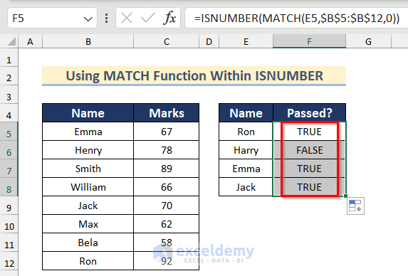
Method 1 – Use MATCH Function Within ISNUMBER Function in Excel
In this method, we’ll use the MATCH function within the ISNUMBER function to match the names from the given list with marks in Excel. Follow these steps:
- Select cell F5 and insert the following formula:
=ISNUMBER(MATCH(E5,$B$5:$B$12,0))- Press Enter and drag down the Fill Handle tool to auto-fill the formula for the rest of the cells.
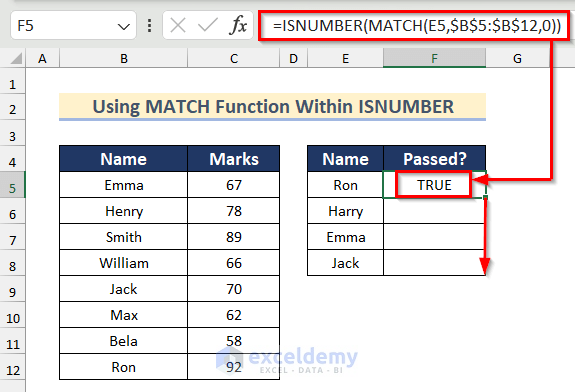
- This will help you determine which student from the list has passed or failed.
How Does the Formula Work?
- We use the MATCH function to find the relative position of the lookup value.
- TWe use the ISNUMBER function to check if the value is a number or not.
Method 2 – Apply IF Function with MATCH & ISNUMBER Functions in Excel
Additionally, we can use the IF function with MATCH and ISNUMBER functions to return a value based on whether the result of ISNUMBER is true or false. Follow these steps:
- In cell C6, insert the following formula:
=IF(ISNUMBER(MATCH(E5,$B$5:$B$12,0)),"Passed","Failed")- Press Enter and drag down the Fill Handle tool for the rest of the cells.
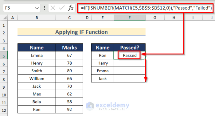
- This will give you results as Passed or Failed in the adjacent cells next to the students’ names.
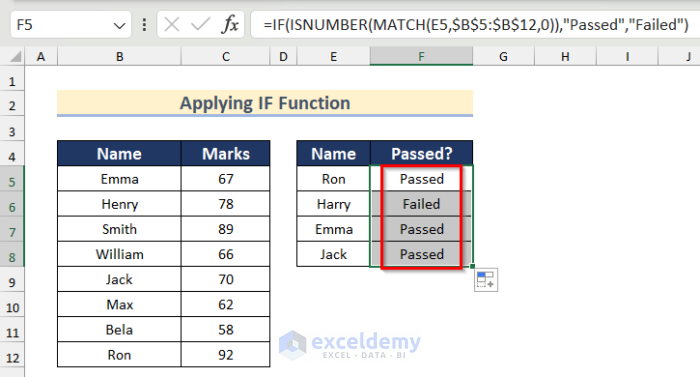
How Does the Formula Work?
- We use the MATCH and ISNUMBER functions to find the value of cell E5 in the cell range B5:B12 and return TRUE if found; otherwise, return FALSE.
- The IF function handles the final output.
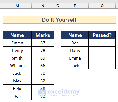
Practice Section
In this section, we are giving you the dataset to practice on your own and learn to use these methods.
Download Practice Workbook
You can download the practice workbook from here:
<< Go Back to Excel Functions | Learn Excel
Get FREE Advanced Excel Exercises with Solutions!

I am trying to use the isnumber and lookup function eg =VALUE(IF(ISNUMBER(VLOOKUP(A5,’Table 1′!$A$4:$P$46,3,FALSE))=TRUE,VLOOKUP(A5,’Table 1′!$A$4:$P$46,3,FALSE),TRIM(MID(A5,2,2))))
when the result is true, but it don’t perform the VLOOKUP(A5,’Table 1′!$A$4:$P$46,3,FALSE);
it alway return the result as TRIM(MID(A5,2,2)).
How to correct it? Thank you
Hello Chan Mau Yin,
It seems like the VLOOKUP inside your ISNUMBER is returning an error or text, not a number that means ISNUMBER(…) is evaluating to FALSE, and that’s why your formula always returns TRIM(MID(…)).
To fix this, make sure the 3rd column of ‘Table 1’!$A$4:$P$46 actually contains numeric values (not text numbers). Also, instead of using ISNUMBER(VLOOKUP(…))=TRUE, simplify the logic using IFERROR like this:
=IFERROR(VALUE(VLOOKUP(A5,’Table 1′!$A$4:$P$46,3,FALSE)), TRIM(MID(A5,2,2)))
This formula tries to return the VLOOKUP result; if it fails (error or not numeric), it falls back to TRIM(MID(…)).
Regards
ExcelDemy
I am using Lookup and Isnumber functions for first time. My column is currency numbers and I want to choose the last row in column H that has a number. I am using this function =LOOKUP(2,1/(ISNUMBER(H:H)),H:H) but getting an error
Hello Sam,
It looks like you’re on the right track!
=LOOKUP(2,1/(ISNUMBER(H:H)),H:H)
This formula normally works to return the last numeric value in column H.
If you’re getting an error, here are a few things to check:
1. Mixed Data Types – Make sure column H only contains numbers and blanks. If there are text values (like “N/A” or spaces), it can cause errors.
2. Array Division – Sometimes Excel doesn’t handle 1/(ISNUMBER(H:H)) well if the range is the entire column. Try limiting it to a practical range, e.g.:
=LOOKUP(2,1/(ISNUMBER(H1:H1000)),H1:H1000)
3. Currency Formatting – If your column looks like currency but is stored as text, ISNUMBER will return FALSE. You may need to convert the text to real numbers first (e.g., use VALUE or re-enter the data).
If after this you still see errors, you can also try:
=LOOKUP(2,1/(H1:H1000<>“”),H1:H1000)
This version finds the last non-blank cell in the range, which often works well for currency data.
Regards,
ExcelDemy