In this tutorial, we’ll unpack the EOMONTH function, how to use it, and how to combine it with other functions.
The screenshot above is an overview of what we’ll cover.
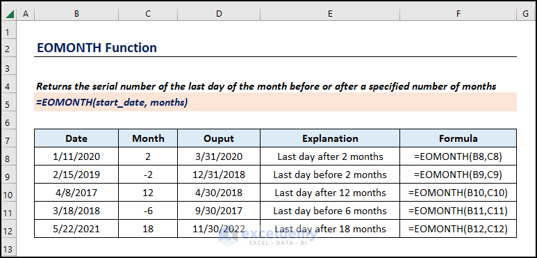
Excel EOMONTH Function: Syntax & Arguments
Function Objective:
The EOMONTH function returns a string of numbers that represent the last day of the month before or after a specified number of months.
Syntax:
=EOMONTH(start_date, months)
Argument Explanation:
| Argument | Required/Optional | Explanation |
|---|---|---|
| start_date | Required | The starting date. |
| months | Required | The number of months prior to or after the starting date. |
Return Parameter:
The last day of the month in the past or future of the specified month.
Version:
The EOMONTH function was introduced in Excel 2007 and is available in all later versions.
How to Use EOMONTH Function in Excel: 10 Ideal Examples
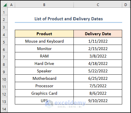
Suppose we have the dataset below containing “Product” and “Delivery Date” columns. Using this dataset, we’ll determine the last days of each month and combine the Excel EOMONTH function with other functions to derive insights from our dataset.
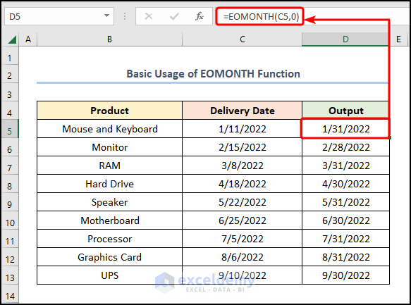
Example 1 – Basic Usage of the EOMONTH Function
Steps:
- In cell D5, enter the EOMONTH function as follows:
=EOMONTH(C5,0)
Here, cell C5 refers to the “Delivery Date” while the 0 (Zero) indicates the present month. The last day of the month in cell C5 is returned.
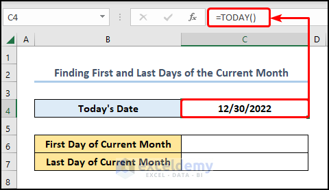
Example 2 – Finding the First and Last Days of the Current Month
Let’s use the EOMONTH function to find the first and last days of the current month.
Steps:
- In cell C4, enter the TODAY function to return today’s date:
=TODAY()
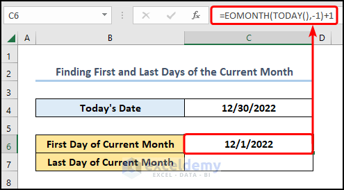
- In cell C6, enter the following formula:
=EOMONTH(TODAY(),-1)+1
In this case, the -1 value prompts the EOMONTH function to yield the last day of the previous month. Adding 1 to the result gives the first date of the current month.
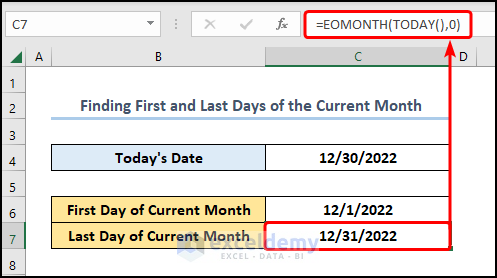
- Enter the following formula in cell C7 to retrieve the last day of the current month:
=EOMONTH(TODAY(),0)
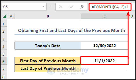
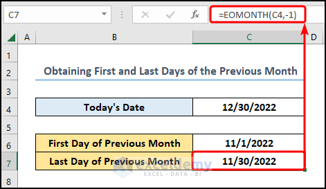
Example 3 – Finding the First and Last Days of the Previous Month
In a similar fashion, we can also compute the first and last days of the previous month.
Steps:
- Get today’s date as shown previously.
- Enter the following formula in cell C6:
=EOMONTH(C4,-2)+1
This function returns the last day of the month 2 months ago, then adds 1 to calculate the first day of the following month, which is this month’s previous month.
- In cell C7 cell, enter the formula below to return the last day of the previous month:
=EOMONTH(C4,-1)
In this case, C4 represents “Today’s Date”.
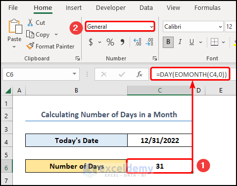
Example 4 – Calculating the Number of Days in a Month
Combining the DAY and EOMONTH functions can be used to return the number of days in a month.
Steps:
- Enter the following formula in cell C6:
=DAY(EOMONTH(C4,0))
- Change the Number Format to General.
The EOMONTH function generates the last day of the month and the DAY function returns the number of days in that month.
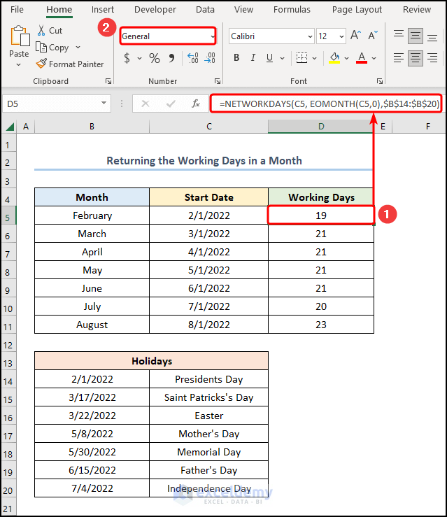
Example 5 – Calculating the Working Days in a Month
By combining the NETWORKDAYS and EOMONTH functions, we can determine the total number of working days in a month.
Steps:
- In cell D5, enter the following formula:
=NETWORKDAYS(C5, EOMONTH(C5,0),$B$14:$B$20)
- Select General as the Number Format.
- NETWORKDAYS(C5, EOMONTH(C5,0),$B$14:$B$20) → returns the number of whole working days between two dates. Here, C5 is the start_date, EOMONTH(C5,0) is the end_date, and the range $B$14:$B$20 represents the optional holidays argument that is referenced from the “Holidays” table.
- Output → 19
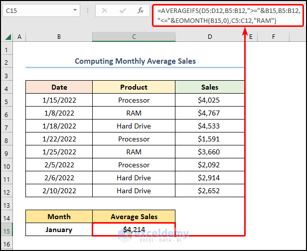
Example 6 – Computing Monthly Average Sales
By applying the AVERAGEIFS and EOMONTH functions together, we can find an average value between two dates based on a condition.
Steps:
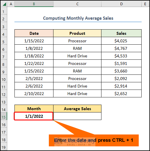
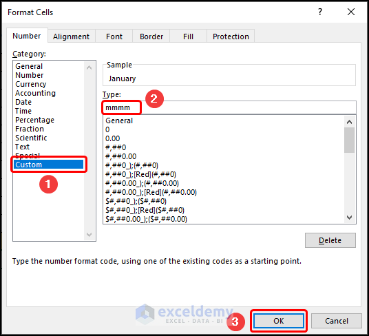
- In the Format Cells window that opens, choose the Custom tab >> type in the code mmmm (a Month Format) >> click OK.
- In cell C15, enter the following formula:
=AVERAGEIFS(D5:D12,B5:B12,">="&B15,B5:B12,"<="&EOMONTH(B15,0),C5:C12,"RAM")
- AVERAGEIFS(D5:D12,B5:B12,”>=”&B15,B5:B12,”<=”&EOMONTH(B15,0),C5:C12,”RAM”) → finds the average for the cells specified by a given set of conditions or criteria. Here, those are:
- D5:D12 is the average_range argument, which is the “Sales” column.
- B5:B12 is the criteria_range1 argument, which refers to the “Date” column, and “>=”&B15 is the criteria1 argument, which is the value greater than or equal to the first day of “January”.
- B5:B12 is the criteria_range2 argument, which refers to the “Date” column, and “<=”&EOMONTH(B15,0) is the criteria2 argument which represents the values less than or equal to the last day of “January”.
- C5:C12 is the criteria_range3 argument, while “RAM” is the criteria3 argument that indicates the “Sales” of “Ram”.
- Output → $4,214
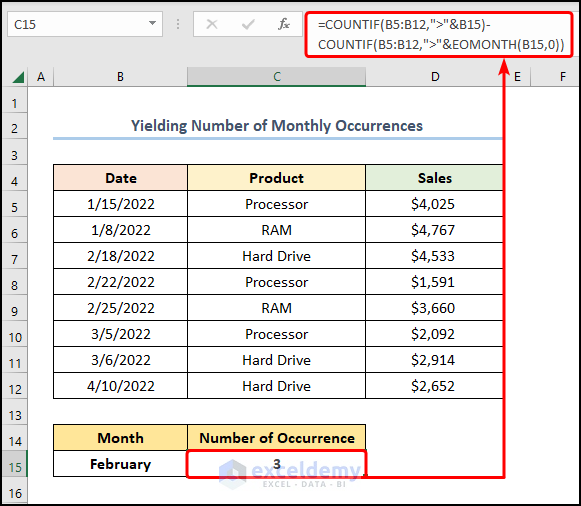
Example 7 – Finding the Number of Monthly Occurrences
We can check for the number of occurrences of a value between two dates by means of the COUNTIF and EOMONTH functions.
Steps:
- Enter the date and apply custom formatting in cell B15 as shown before.
- Copy and paste the following formula into cell C15:
=COUNTIF(B5:B12,">"&B15)-COUNTIF(B5:B12,">"&EOMONTH(B15,0))
- COUNTIF(B5:B12,”>”&B15) → counts the number of cells within a range that meet the given condition. Here, B5:B12 represents the range argument that refers to the Date column, while “>”&B15 indicates the criteria argument that returns the count of the matched value.
- Output → 6
- COUNTIF(B5:B12,”>”&EOMONTH(B15,0)) → here, B5:B12 represents the range argument that refers to the Date column, while “>”&EOMONTH(B15,0) indicates the criteria argument that returns the count of the matches.
- Output → 3
- COUNTIF(B5:B12,”>”&B15)-COUNTIF(B5:B12,”>”&EOMONTH(B15,0)) → becomes
- 6 – 3 → 3
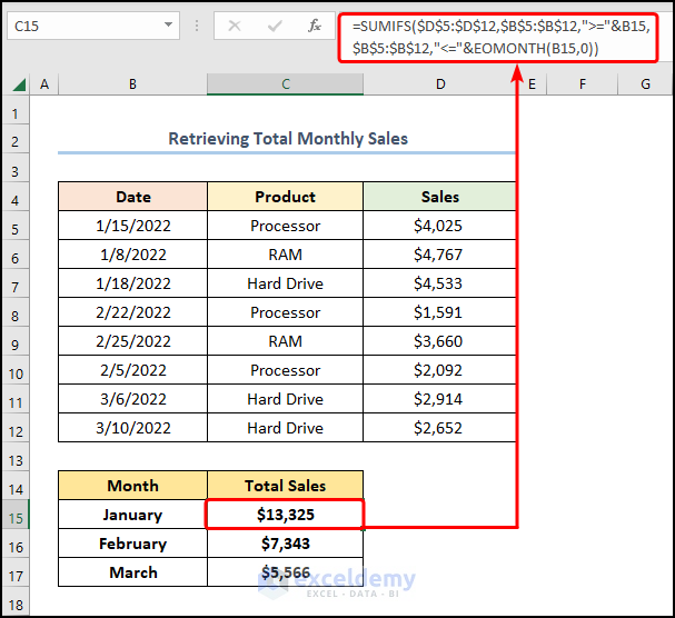
Example 8 – Retrieving Total Monthly Sales
We can also determine the “Total Sales” using the SUMIFS and EOMONTH functions
Steps:
- Follow the steps above to enter the formatted month names in cells B15:B17.
- Enter the following formula in cell C15:
=SUMIFS($D$5:$D$12,$B$5:$B$12,">="&B15,$B$5:$B$12,"<="&EOMONTH(B15,0))
- SUMIFS($D$5:$D$12,$B$5:$B$12,”>=”&B15,$B$5:$B$12,”<=”&EOMONTH(B15,0)) → adds the cells specified by a given set of conditions or criteria. Here, $D$5:$D$12 is the sum_range argument that refers to the “Sales” column, $B$5:$B$12 represents the criteria_range_1 argument that points to the “Date” column, and “>=”&B15 is the criteria_1 argument representing the values greater than or equal to the first day of “February”. Next, $B$5:$B$12 is the criteria_range_2 argument which indicates the “Date” column and “<=”&EOMONTH(B15,0) is the criteria_2 argument representing the values less than or equal to the last day of “February”.
- Output → $13,325
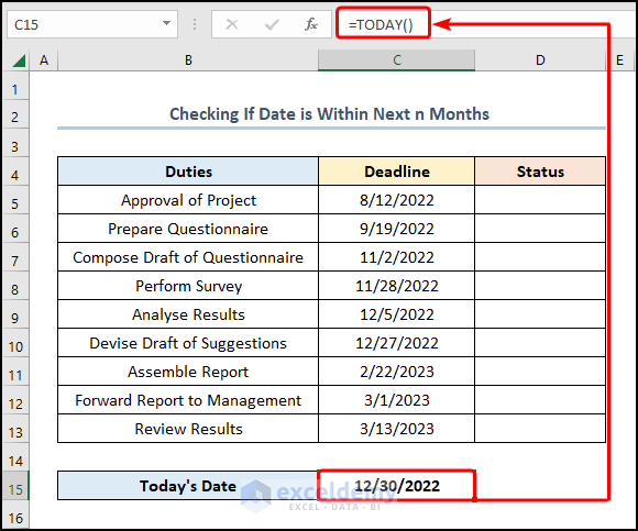
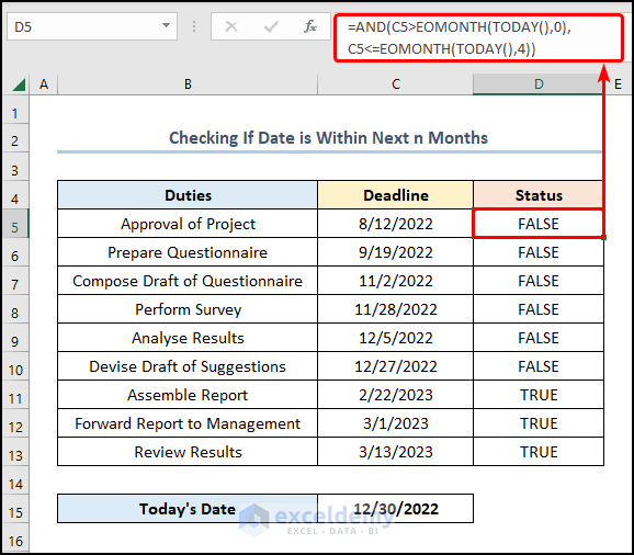
Example 9 – Checking If a Date Is Within the Next n Months
We can use the AND function in conjunction with the EOMONTH function to check if a date is within the next n months. Here, we’ll set the n to 4 months in the future.
Steps:
- Enter the TODAY function in cell C15:
=TODAY()
- Enter the formula below in cell D5:
=AND(C5>EOMONTH(TODAY(),0),C5<=EOMONTH(TODAY(),4))
- AND(C5>EOMONTH(TODAY(),0),C5<=EOMONTH(TODAY(),4)) → checks whether all the arguments are TRUE, and returns TRUE if they are. C5>EOMONTH(TODAY(),0) is the logical1 argument that checks if the date in cell C5 is greater than today’s date, and C5<=EOMONTH(TODAY(),4) is the logical2 argument that checks whether the date in cell C5 is less than the last day of the month 4 months in the future. Since the first argument is FALSE and the second argument is TRUE, the AND function returns the output FALSE.
- Output → FALSE
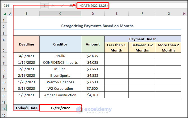
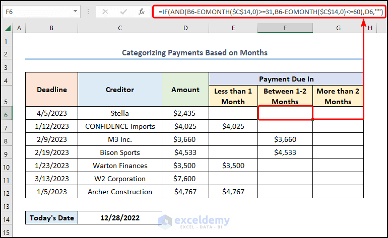
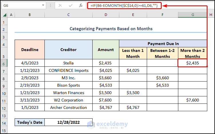
Example 10 – Categorizing Payments Based on Months
We can prioritize outstanding payments by grouping them with the IF, DATE, and EOMONTH functions.
Steps:
- Enter the DATE function below in cell C14 to obtain today’s date:
=DATE(2022,12,28)
In this case, 2022, 12, and 28 point to the year, month, and day arguments respectively.
Note: You can open the Format Cells dialog box by pressing CTRL + 1 and change the cell formatting to Short Date.
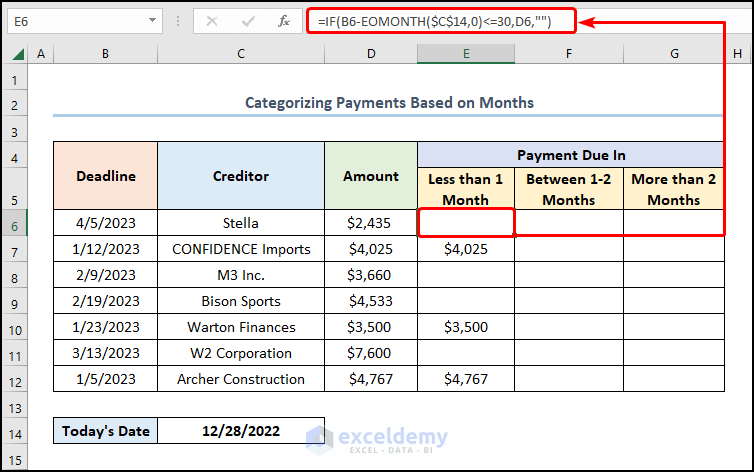
- In cell E6, enter the formula below, press Enter, then drag the Fill Handle tool to copy the formula to the cells below:
=IF(B6-EOMONTH($C$14,0)<=30,D6,"")
- EOMONTH($C$14,0) → returns the serial number of the last day of the month before or after a specified number of months. Here, C14 is the start_date argument, and 0 (zero) is the months argument, representing the current month.
- Output → 12/31/2022
- IF(B6-EOMONTH($C$14,0)<=30,D6,””) → checks whether a condition is met and returns one value if TRUE and another value if FALSE. Here, B6-EOMONTH($C$14,0)<=30 is the logical_test argument that checks if the difference between the dates B6-EOMONTH($C$14,0) is less than or equal to 30. If true, the function returns D6 (the value_if_true argument), otherwise it returns “” (Blank) (the value_if_false argument).
- Output → “” (Blank)
- In cell F6, enter the formula below:
=IF(AND(B6-EOMONTH($C$14,0)>=31,B6-EOMONTH($C$14,0)<=60),D6,"")
- AND(B6-EOMONTH($C$14,0)>=31,B6-EOMONTH($C$14,0)<=60) → Here, B6-EOMONTH($C$14,0)>=31 is the logical1 argument that checks if the difference between the two dates is greater than 31, and B6-EOMONTH($C$14,0)<=60 is the logical2 argument that checks whether the difference between the two dates is less than 60. Since the first argument is TRUE and the second argument is FALSE, the AND function returns FALSE.
- Output → FALSE
- IF(AND(B6-EOMONTH($C$14,0)>=31,B6-EOMONTH($C$14,0)<=60),D6,””) → becomes
- IF(FALSE,D6,””) → The FALSE value of the logical_test argument prompts the function to return “” (Blank) (value_if_false argument).
- Output → “” (Blank)
- Enter the following formula in cell G6:
=IF(B6-EOMONTH($C$14,0)>=61,D6,"")
How to Determine the End Date of a Future Month Using EoMonth in Excel VBA
Last but not least, we can determine the end date of a future month using the EoMonth function in VBA. On this occasion, we’ll compute the last date of the month 6 months into the future.
Steps:
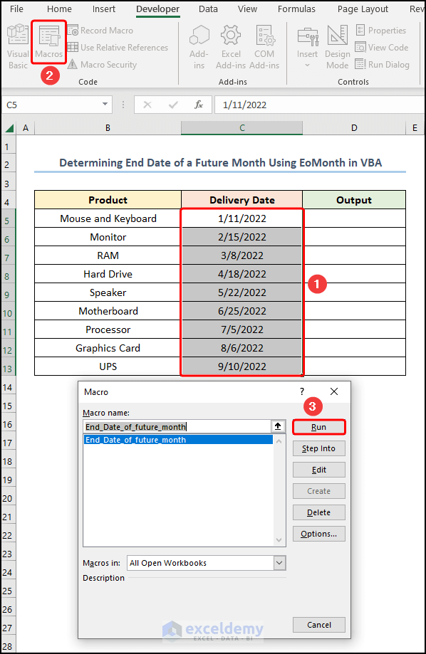
- Go to the Developer tab >> click the Visual Basic button.
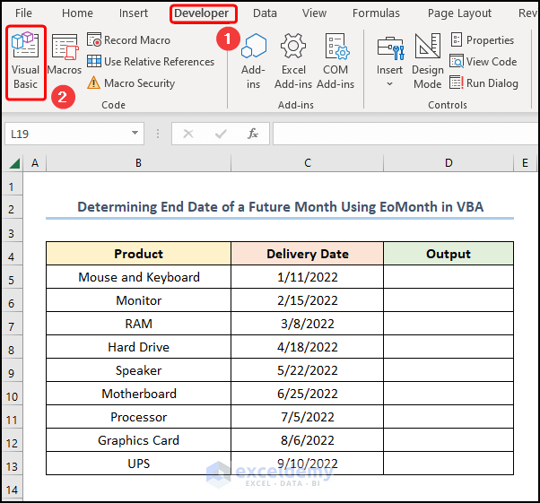
The Visual Basic Editor opens in a new window.
- Go to the Insert tab >> select Module.
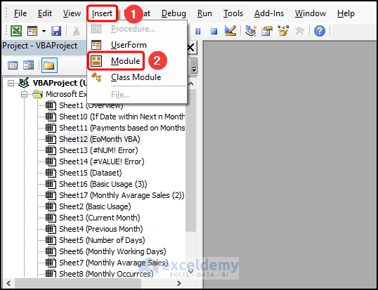
Copy the code below and paste it into the window:
Sub End_Date_of_future_month()

Dim r_range As Range
Set r_range = Selection
Dim selected_cells As Range

For Each selected_cells In r_range
 selected_cells.Offset(0, 1) = Application.WorksheetFunction.EoMonth(selected_cells, 6)
Next selected_cells

End Sub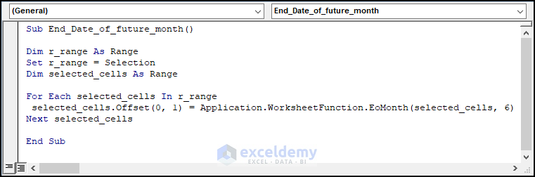
- In the first portion, the sub-routine is given a name, End_Date_of_future_month().
- Next, the variables r_range and selected_cells are defined and assigned as type Range.
- A For Loop is used to iterate through the cells in the r_range while applying the EoMonth function to return the end date and the Offset property to paste the results into the adjacent column.
- Close the VBA window >> select the range C5:C13 >> click the Macros button >> hit Run.
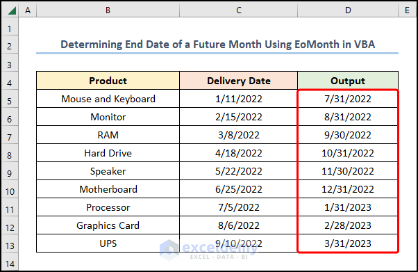
The results should look like the screenshot below.
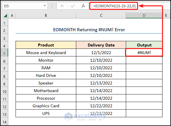
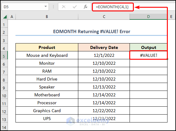
Common Errors While Using the EOMONTH Function in Excel
There are several errors we may encounter while using the EOMONTH function.
| Error | Reason |
|---|---|
| #NUM! | The start_date argument is an invalid date. |
| #VALUE! | The start_date argument is text. |
- The function will return the #NUM! Error if the start_date argument contains an invalid Date format, like “23-23-22”.
- Additionally, we will face the #VALUE! Error if the start_date argument is a non-numeric value, for instance, cell C4 refers to the text “Delivery Date”.
Things to Remember
- A positive number in the months argument returns dates in the future, whereas a negative number yields dates in the past.
- The EOMONTH function ignores any decimal values given in the start_date and months arguments.
- By default, the EOMONTH function generates the date as a serial number that needs to be formatted as a Date.
Download Practice Workbook
<< Go Back to Excel Functions | Learn Excel
Get FREE Advanced Excel Exercises with Solutions!
