Method 1 – Using Single Criteria for Equal in Value in AVERAGEIFS Function
Steps:
- Type the following formula in cell H6.
=AVERAGEIFS(C6:C23,E6:E23,"Won")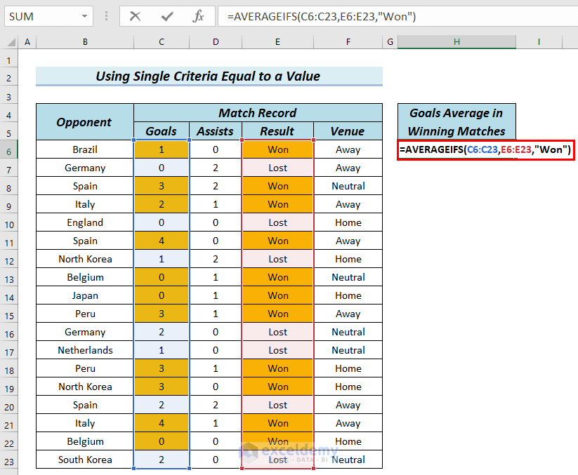
Formula Breakdown
- AVERAGEIFS(C6:C23,E6:E23,”Won”) → Calculates the average of only those cells in the array C6 to C23 which corresponding cells in the array E6 to E23 contain “Won”.
- Output: 2.09
- Press ENTER.
See the result in cell H6.

Method 2 – Use of Single Criteria for Blank Cells
Steps:
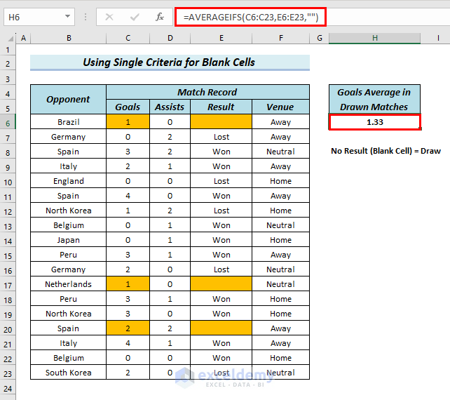
- Type the following formula in cell H6.
=AVERAGEIFS(C6:C23,E6:E23,"")Formula Breakdown
- AVERAGEIFS(C6:C23, E6:E23,””) → Calculates the average of only those cells in the array C6 to C23 which corresponding cells in the array E6 to E23 are blank.
- Output: 1.33
- Press ENTER.
See the result in cell H6.
Method 3 – Use of Single Criteria for Cells That Are Not Blank
Steps:
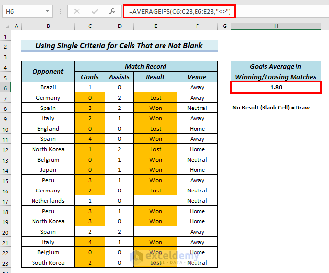
- Type the following formula in cell H6.
=AVERAGEIFS(C6:C23,E6:E23,"<>")Formula Breakdown
- AVERAGEIFS(C6:C23, E6:E23,”<>”) → Calculates the average of only those cells in the array C6 to C23 which corresponding cells in the array E6 to E23 are not blank.
- Output: 1.80
- Press ENTER.
See the result in cell H6.
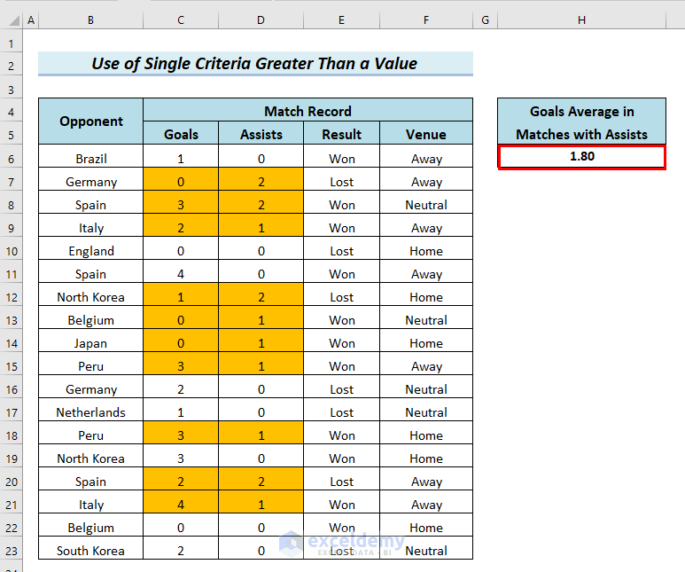
Method 4 – Use of Single Criteria for Greater Than Value
Steps:
- Type the following formula in cell H6.
=AVERAGEIFS(C6:C23,D6:D23,">=1")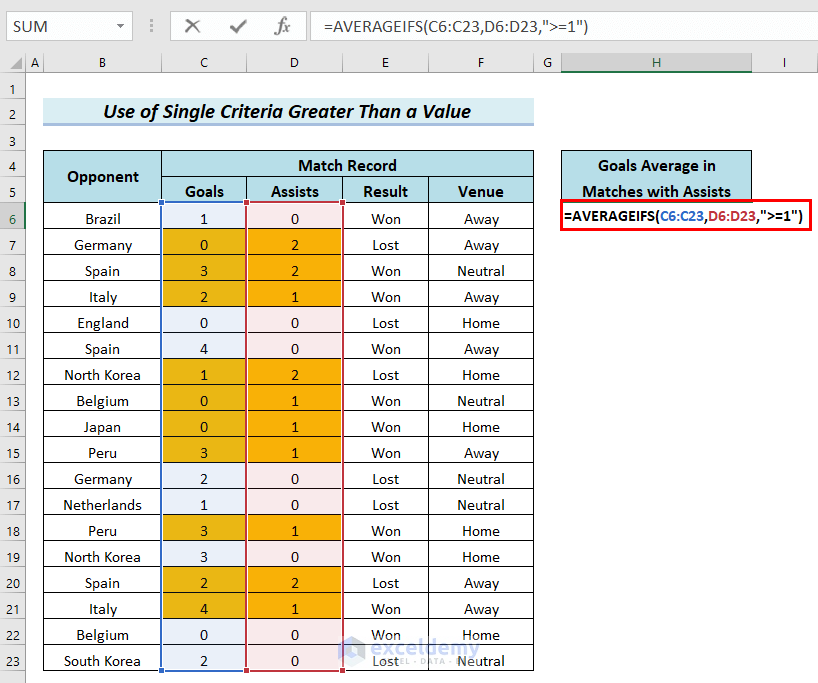
Formula Breakdown
- AVERAGEIFS(C6:C23,D6:D23,”>=1″) → Calculates the average of only those cells in the array C6 to C23 which corresponding cells in the array D6 to D23 contain anything greater than or equal to 1.
- Output: 1.80
- Press ENTER.
See the result in cell H6.
Method 5 – Applying Multiple Criteria in the AVERAGEIFS Function
Steps:
- Type the following formula in cell H6.
=AVERAGEIFS(C6:C23,C6:C23,">=1",F6:F23,"Home")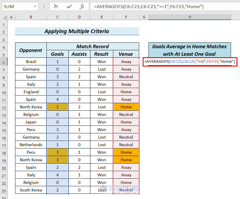
Formula Breakdown
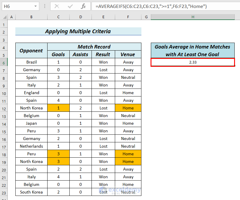
- AVERAGEIFS(C6:C23,C6:C23,”>=1″,F6:F23,”Home”) → Calculates the average of only those cells in the array C6 to C23 that contain anything greater than or equal to 1 and which corresponding cells in the array F6 to F23 contain “Home”.
- Output: 2.33
- Press ENTER.
See the result in H6.
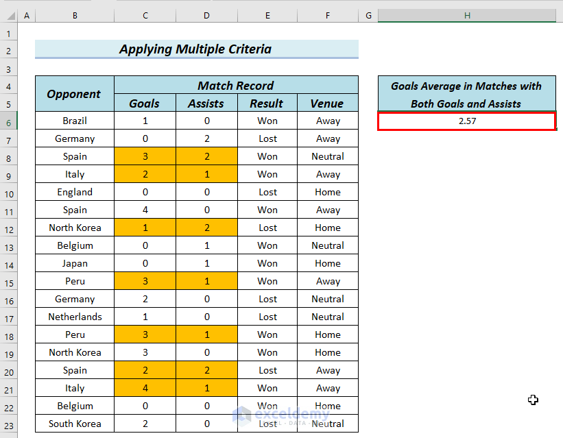
Find out the average of goals when the Goals number is greater than or equal to 1 and when the Assists number is greater than or equal to 1. We marked both criteria with Yellow.
- Type the following formula in cell H6.
=AVERAGEIFS(C6:C23,C6:C23,">=1",D6:D23,">=1")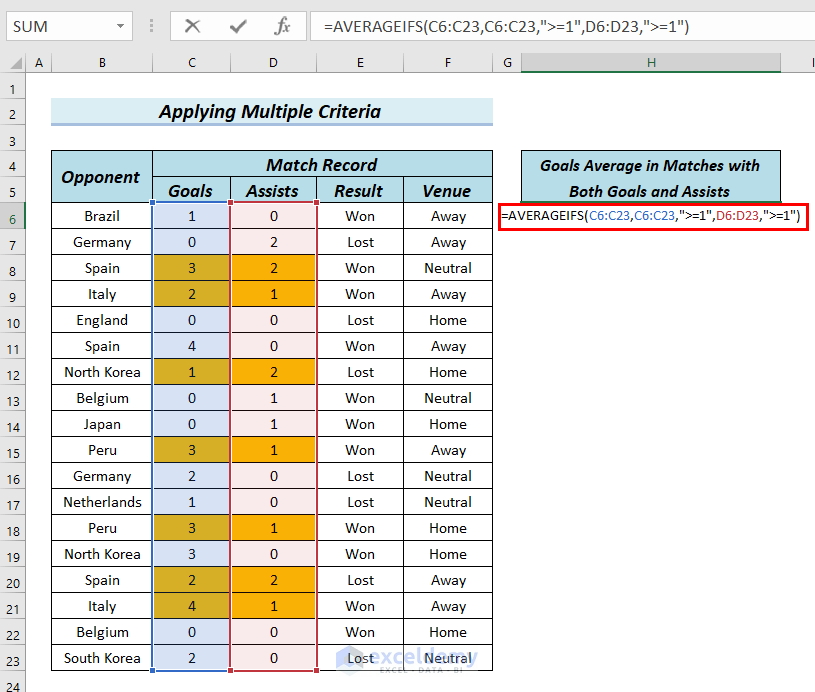
Formula Breakdown
- AVERAGEIFS(C6:C23,C6:C23,”>=1″,D6:D23,”>=1″) → Calculates the average of only those cells in the array C6 to C23 that contain anything greater than or equal to 1 and which corresponding cells in the array D6 to D23 contain anything than or equal to 1.
- Output: 2.33
- Press ENTER.
See the result in H6.
Method 6 – Counting Average with Partial Match (Wildcard Character)
Steps:
- Type the following formula in cell H6.
=AVERAGEIFS(C6:C23,B6:B23,"*Korea")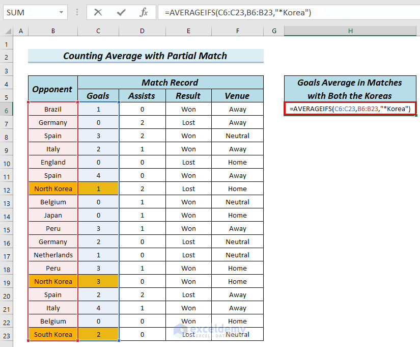
Formula Breakdown
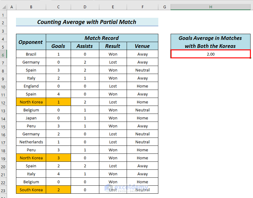
- AVERAGEIFS(C6:C23,B6:B23,”*Korea”) → Calculates the average of only those cells in the array C6 to C23 which corresponding cells in the array B6 to B23 contain anything having “Korea” at the end.
- Output: 2
- Press ENTER.
See the result in cell H6.
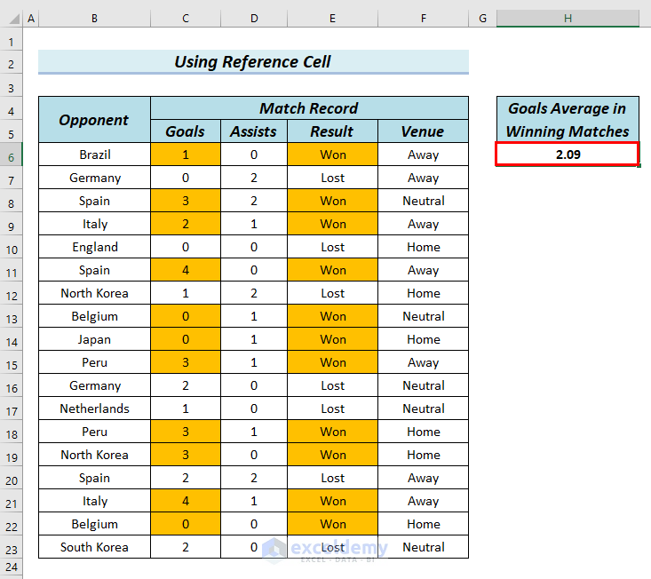
Method 7 – Using Cell References in AVERAGEIFS Function
Steps:
- Type the following formula in cell H6.
=AVERAGEIFS(C6:C23,E6:E23,E6)
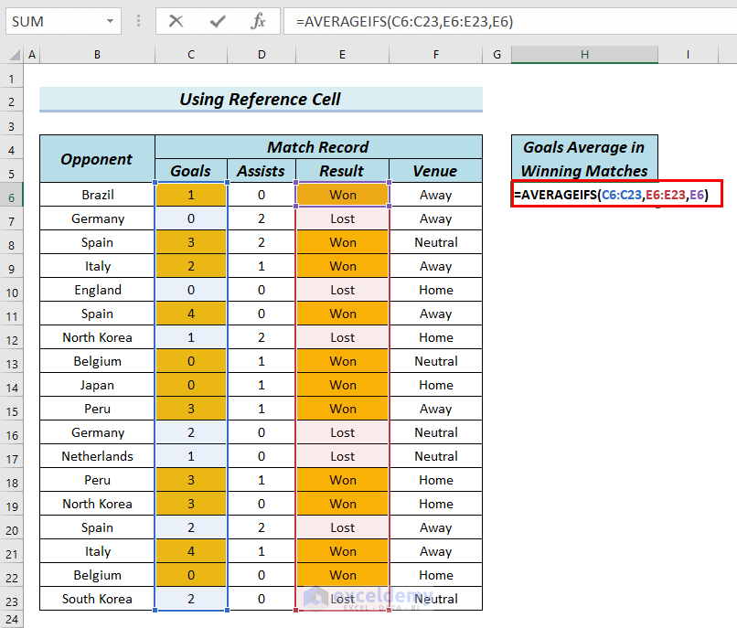
Formula Breakdown
- AVERAGEIFS(C6:C23,E6:E23,E6) → Calculates the average of only those cells in the array C6 to C23 which corresponding cells in the array E6 to E23 contain the cell content of cell E6 that is “Won”.
- Output: 2.09
- Press ENTER.
See the result in cell H6.
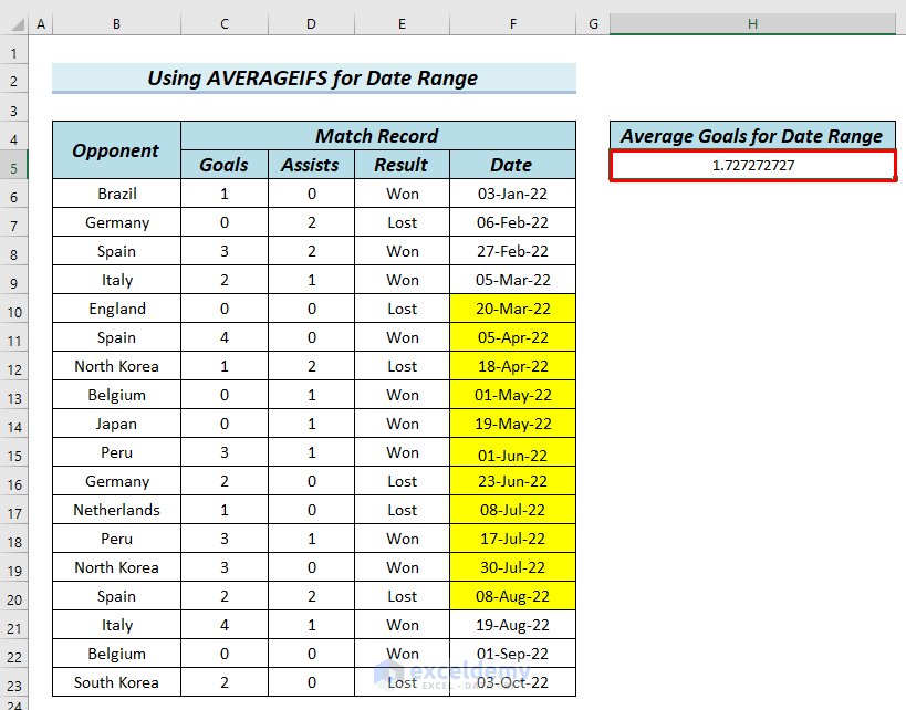
Method 8 – Applying Date Range in AVERAGEIFS Function
Steps:
- Type the following formula in cell H6.
=AVERAGEIFS(C6:C23,F6:F23,"<=8-Aug-22",F6:F23,">=20-Mar-22")
Formula Breakdown
- AVERAGEIFS(C6:C23,F6:F23,”<=8-Aug-22″,F6:F23,”>=20-Mar-22″) → Calculates the average of only those cells in the array C6 to C23 which corresponding cells in the array F6 to F23 contain dates greater than or equal to 20-Mar-22 and less than or equal to 8-Aug-22.
- Output: 1.727272727
- Press ENTER.
See the result in H6.
Common Errors with Excel AVERAGEIFS Function
In the following table, we showed the common errors of the AVERAGEIFS function and the reasons for such errors.
| Error | When They Show |
|---|---|
| #DIV/0! | Shows when no value in the average_match matches all criteria. |
| #VALUE! | This shows when the lengths of all the arrays are not the same. |
Things to Remember
- The AVERAGEIFS function ignores blank or empty cells. If a cell in the average_range is blank or contains text, it won’t be included in the average calculation, even if it meets the specified criteria.
- If no cells meet the specified criteria, the AVERAGEIFS function returns the #DIV/0! Error. You can use error handling techniques, such as the IFERROR function, to display a custom message or handle the error gracefully.
- The ranges specified in criteria_range1, criteria_range2, etc., must be the same size as the average_range. If they are not the same size, the function will return an error.
Frequently Asked Questions
- What is the difference between the Averageif() and Averageifs() functions?
AVERAGEIF() is used for single criterion averaging, while AVERAGEIFS() allows for averaging based on multiple criteria
- Is it possible to use logical operators, such as “AND” or “OR,” within the criteria of the AVERAGEIFS function in Excel to combine multiple conditions for averaging?
Use logical operators within the criteria of the AVERAGEIFS function in Excel to combine multiple conditions for averaging. Use the “AND” operator to specify that all the conditions must be met or the “OR” operator to specify that any conditions can be met.
Download Practice Workbook
You can download the following Excel file and practice while reading this article.
Excel AVERAGEIFS Function: Knowledge Hub
<< Go Back to Excel Functions | Learn Excel
Get FREE Advanced Excel Exercises with Solutions!
