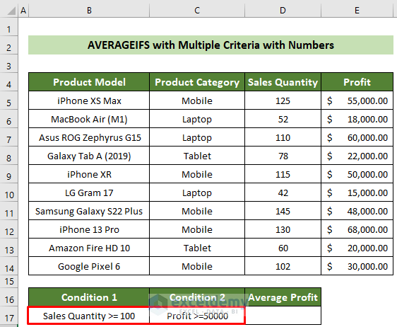
Method 1 – AVERAGEIFS for Multiple Criteria with Numbers
Steps:
- Specify your conditions in cells B17 and C17 for better visualization.
- Click on cell D17.
- Insert the following formula and press the Enter key.
=AVERAGEIFS(E5:E14,D5:D14,">=100",E5:E14,">=50000")
Get the average profit for only the products that have sales quantity greater than or equal to 100 and profit is greater than or equal to 50000.
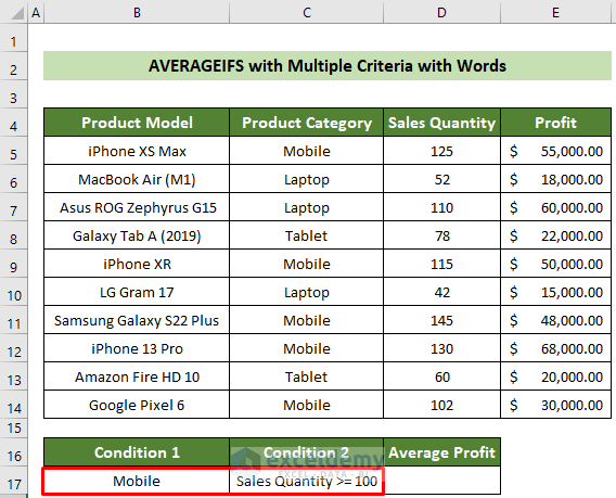
Method 2 – AVERAGEIFS with Words Criteria
Steps:
- Record your conditions in cells B17 and C17.
- Click on cell D17 and insert the following formula.
=AVERAGEIFS(E5:E14,C5:C14,"Mobile",D5:D14,">=100")- Hit the Enter key.
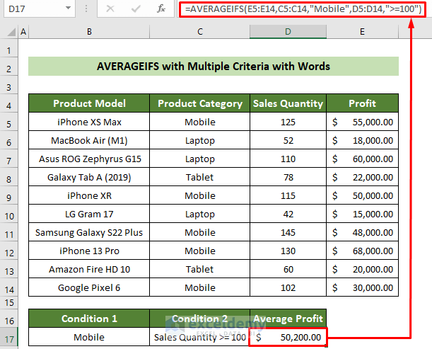
Achieve your desired result in cell D17.
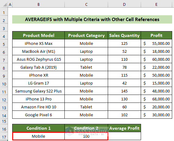
Method 3 – Multiple Criteria with Other Cell References
Steps:
- Record your conditions in cells B17 and C17.
- Put the condition values only.
- Click on cell D17.
- Insert the following formula and press the Enter key.
=AVERAGEIFS(E5:E14,C5:C14,B17,D5:D14,">="&C17)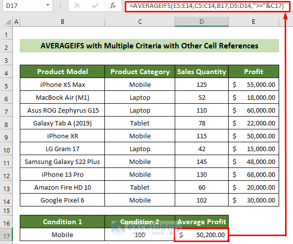
Get your required filtered average in cell D17.
Method 4 – Multiple Criteria with Partially Matched Words
Steps:
- Record the conditions in cells B17 and C17.
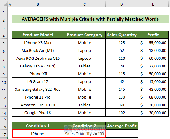
- Click on cell D17 and insert the following formula.
=AVERAGEIFS(E5:E14,B5:B14,"iPhone*",D5:D14,">=100")- Hit the Enter key.
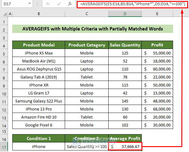
Get the required average profit for iPhones that have sales quantity greater than or equal to 100.
Excel AVERAGE with Multiple OR Criteria in the Same Range
Steps:
- Record your conditions first in cells B17 and C17.
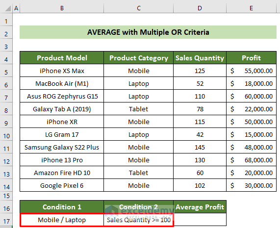
- Click on cell D17 and insert the following formula.
=AVERAGE(IF((C5:C14={"Mobile","Laptop"})*(D5:D14>=100),E5:E14))- Press the Ctrl + Shift + Enter key.
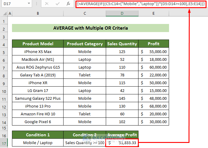
Get the desired average result for your OR conditions.
Things to Remember
- If no cell matches your given criteria in the AVERAGEIFS function, the function will return the #DIV0! error.
- You need to put your non-numeric criteria inside double quotes(“ ”).
- The criteria ranges and average range has to possess the same number of rows and columns.
Download Practice Workbook
You can download our practice workbook from here for free!
Related Article
<< Go Back to Excel AVERAGEIFS Function | Excel Functions | Learn Excel
Get FREE Advanced Excel Exercises with Solutions!

Hello there!
Need some help with a somewhat complex formula (I think?). I’m trying to find the average of two separate criteria from the same column in one sheet while also making it date specific using the EOMONTH function from another sheet where the date is defined in it’s cell.
Just FYI – This below formula works as an array perfectly however when I attempt to borrow/copy the EOMONTH portion from another formula that works (further down below) it it no longer works. I believe I just simply do not understand the right combination or order to combne everything together.
=AVERAGE(IF(ISNUMBER(MATCH(‘ONLINE MASTER’!F2:F10000,{“TELEPHONE”,”COMPUTER”},0)),’ONLINE MASTER’!D2:D10000))
More Info: I am plugging these formulas in on one sheet but the bulk of the criteria is found on one sheet while the date specific info lives on the second sheet. Here is all the sheet/column info for both and what each represents:
Sheet Names
ONLINE MASTER = Sheet 1
2022 = Sheet 2
Column’s in Sheet 1 “ONLINE MASTER”:
Column A = Where all the dates are (data exists in cells A2-A10000)
Column D = The numbers I need to average (data exists in cells D2-D10000)
Column F = Different sets of category items (i.e. PHONE, COMPUTER, STAPLER, SCISSORS)(data exists in cells F2-F10000)
Column’s in Sheet 2 “2022” (where the formula is intended to go):
Column A = data where all preset dates are in Month-Year format (i.e. Oct-22)
Another formula on sheet 2: “2022” where the EOMONTH formula works is a follows:
=IFERROR(ROUND(AVERAGEIFS(‘ONLINE MASTER’!$D$2:$D$10000, ‘ONLINE MASTER’!F2:F10000,”COMPUTER”,’ONLINE MASTER’!$A$2:$A$10000,”>=”&EOMONTH($A$63,-1)+1,’ONLINE MASTER’!$A$2:$A$10000,”<="&EOMONTH($A$63,0)),2),0)
In the above formula A63 represents October 2022 and the formula calculates the average of all computers sold in the month of October based on their respective prices.
All months in the year also live defined in column A and I'm sure if you could please help me with this one formula it will unlock all the other formulas as well.
Thanks in advance!
Hello, CRYSTAL!
Thank you for your query.
As far as I understood your question, you want to apply date criteria and multiple Category criteria in your formula to find the average of a different column.
You can accomplish this using the nested FILTER function along with the AVERAGE, EOMONTH, and DAY functions and you have to use the plus sign between the categories to enable the OR criteria. The final formula would look like this.
=AVERAGE((FILTER('ONLINE MASTER'!$D$2:$D$1000,(('ONLINE MASTER'!$F$2:$F$1000="COMPUTER")+('ONLINE MASTER'!$F$2:$F$1000="TELEPHONE"))*('ONLINE MASTER'!$A$2:$A$1000>=('2022'!$A63-DAY('2022'!$A63)+1))*('ONLINE MASTER'!$A$2:$A$1000<=EOMONTH(('2022'!$A63-DAY('2022'!$A63)+1),0)))))I hope this solves your problem.
With Regards,
Md. Tanjim Reza Tanim
I found that you can use a=verage(averageif(;;);averageif(;;)) or you can use a=verage(averageifs(;;;;);averageifs
(;;;;))
Thank you, Hossam for your query. I am not sure whether you alter AVERAGEIF with AVERAGEIFS. If so, there should be a difference between them as AVERAGEIF deals with single criterion whereas AVERAGEIFS deals with multiple criteria. However, you can use the AVERAGEIFS function for a single criterion by specifying only one criterion range and one criterion. For example, you have a range of cells A1:A10 that contains numbers and you want to calculate the average of the cells that are greater than or equal to 5. For accomplish your task, you can use the AVERAGEIFS function like this:
=AVERAGEIFS(A1:A10, A1:A10, ">=5")Further if you have any query, please let me know. Thank you.
I’ve looked at several sites and this is where I found what I needed. I don’t know if it’s the wording I’ve used but I could not find this last part anywhere else ‘Excel AVERAGE with Multiple OR Criteria in the Same Range’.
Thank you.
Hello ZAC!
Thanks for sharing your problem with us!
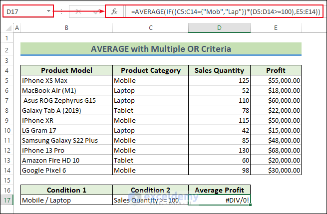
You’ve used the wording but could not find this last part anywhere else ‘Excel AVERAGE with Multiple OR Criteria in the Same Range’.
The formula returns #DIV/0! error because the matching values are different from the data table.
You can fix the issue using the following formula with a partial match.
Please download the Excel file for solving your problem and practice with it.
Excel AVERAGEIFS with Multiple Criteria in Same Range
If you cannot solve your problem, please mail us at the address below.
[email protected]
Regards
Md. Abdur Rahim Rasel
Exceldemy Team