Latest Posts From Tanjim Reza

Method 1 - Break-Even Units: This is the unit that you need to sell to reach your break-even point. Break Even Units = ...
![Excel Payment Calculator [Free Download]](https://www.exceldemy.com/wp-content/uploads/2023/12/4.-Excel-Payment-Calculator.png)
Excel payment calculator is one of the most common and essential calculators to track and plan various loan or savings payments. In this free downloadable ...

How to Create a Budget in Excel: Knowledge Hub How to Create a Personal Budget in Excel How to Make a Personal Monthly Budget in Excel How to Make ...

A bank statement is a list of records of transactions between a bank and its account holders. It is provided upon valid requests of any account holder of a ...
![ARM Amortization Schedule Excel Template [Free Download]](https://www.exceldemy.com/wp-content/uploads/2023/12/1-arm-amortization-schedule-excel-template.png?v=1701945344)
Instructions: Open the ARM Amortization Schedule template and insert all the required inputs in the blue-shaded area of the Input Values column. The ...
![Excel Quarterly Amortization Schedule [Free Download]](https://www.exceldemy.com/wp-content/uploads/2023/12/1-Quarterly-Amortization-Schedule-Template.png?v=1701754819)
The quarterly amortization schedule is a helping tool to track one’s quarterly loan repayment process. It is assumed that the borrower pays his payments ...
![Excel Monthly Amortization Schedule [Free Download]](https://www.exceldemy.com/wp-content/themes/rehub-theme/images/default/blank.gif)
Download our free Excel Monthly Amortization Schedule template to generate your monthly amortization schedule and read the article to learn how to use this ...
![Excel Bi-Weekly Amortization Schedule [Free Download]](https://www.exceldemy.com/wp-content/uploads/2023/12/1-Bi-weekly-amortization-schedule-template.png?v=1701752127)
A bi-weekly amortization schedule is a great tool to visualize one’s bi-weekly loan repayment process. From this schedule, s/he will be able to know how much ...
![Excel Weekly Amortization Schedule [Free Download]](https://www.exceldemy.com/wp-content/uploads/2023/12/1-Weekly-Amortization-Schedule-Template.png?v=1701684181)
Amortization schedule is a visualization tool that helps borrowers keep track of their loan repayment process over the loan term. For the weekly amortization ...
![How to Use the Excel Student Loan Amortization Schedule [Free Download]](https://www.exceldemy.com/wp-content/uploads/2023/11/8-Student-Loan-Amortization-Schedule-with-Grace-Period.png?v=1701168840)
Download the Free Excel Student Loan Amortization Schedule Template Feel free to download our free Excel Student Loan Amortization Schedule template. This ...
![Excel 30 Year Amortization Schedule Template [Free Download]](https://www.exceldemy.com/wp-content/uploads/2023/11/1-30-year-amortization-schedule-template.png?v=1700987892)
Download our free 30-Year Amortization Schedule Excel template to generate your own amortization schedule for a 30-year loan. Read the article carefully to ...
![Excel Car Loan Amortization Schedule Template [Free Download]](https://www.exceldemy.com/wp-content/uploads/2023/11/1-Car-Loan-Amortization-Schedule-Template.png?v=1700724005)
This template will be helpful to bankers, business owners, job holders, financial planners, and all kinds of lenders and borrowers looking to take or give away ...
![Excel Actual/360 Amortization Calculator Template [Free Download]](https://www.exceldemy.com/wp-content/uploads/2023/11/1-Actual-360-Amortization-Calculator.png?v=1700639866)
The Actual/360 amortization calculator is a great tool to visualize one’s loan repayment process when interest is calculated while considering the actual ...
![Multiple Loan Amortization Schedule Excel Template [Free Download]](https://www.exceldemy.com/wp-content/uploads/2023/11/1-Multiple-Loan-Amortization-Schedule-Excel-Template.png?v=1700034706)
How to Use This Template Instructions: Open the file and go to the Loan Input sheet. Insert your multiple loan parameter values and choose the required ...

In the Amortization schedule borrowers can visualize their loan repayment process. This schedule shows: regular due payment, principal paid, interest paid, and ...
- 1
- 2
- 3
- …
- 10
- Next Page »
See Our Reviews at


Hello, ENG NICHOLAS LUMANYIKA!
You are welcome.
About your query, yes, if you do not have any taxes and other costs associated with your vehicle, you can leave those cells blank. The given formula will analyze your vehicle life cycle accordingly.
With Regards,
Md. Tanjim Reza Tanim
Team Leader, ExcelDemy
Hello, Nicholas Lumanyika!
Thank you so much for your valuable feedback.
Yes, you are right. The total cost of 45*5 would be for 100 km. So, In this calculation, we have to find our total fuel cost per vehicle first. Then we have to divide the total fuel cost by total fuel consumption. So, the final formula in the D21 cell would be:
=((D19/100)*D17*D20)/D17
We have corrected the file and formula of our article accordingly. Please check it now and use the file as you need.
If you have any further queries, confusion, or recommendation please feel free to reach out to us.
With Regards,
Md. Tanjim Reza Tanim
Team Leader, ExcelDemy.
Hello, Nicholas Lumanyika!
Thank you for your query.
Regarding your query, Acquisition cost in vehicle life cycle cost analysis refers to the initial cost incurred when purchasing a vehicle. It includes the total expenses associated with acquiring the vehicle, such as the actual purchase price, taxes, licensing fees, delivery charges, and any additional costs directly related to the procurement of the vehicle.
So, if you had to pay tax and other subsidies when purchasing the vehicle, you must enlist these in the acquisition cost calculation.
And, regarding your second query, yes, maintenance cost include both scheduled and unscheduled maintenance costs.
With Regards,
Md. Tanjim Reza Tanim
Team Leader, ExcelDemy
Hello, Sachin!
Thank you for your query. Regarding your query, this article was written based on the 2023 regime. But, the TDS calculator basics are the same for every regime. Only the variables, like tax deduction percentage, education cess percentage, etc. can change from year to year which would slightly affect the calculation. But, the basics are the same. So, it’s better if you check your current tax variable percentages for this regime in your region and use our file accordingly.
Hopefully, you will be able to use the file in your calculation properly.
With Regards,
Md. Tanjim Reza Tanim
Team Leader, Exceldemy
Hello, TANVIR!
Thank you for your query. Regarding your query, to get a home loan emi calculator with floating interest rates, you will need a new mortgage calculator where interest rates vary.
To help you, I can link you to another of our tutorials which exactly will serve your needs.
https://www.exceldemy.com/loan-amortization-schedule-excel-with-variable-interest-rate/
Please download the template from the above link and go through the article to learn how to use it. Hope, it will help.
Regards,
Md. Tanjim Reza Tanim
Hello, PREM! Hope you are doing well.
Thank you for your query.
Regarding your query, basically, the Balance Sheet comes after generating a journal, ledger, trial balance, income statement, and owner’s equity statement. So, to automate a balance sheet, you need to automate journal, ledger, trial balance, income statement, and owner’s equity statement first.
In this article, basically, we automated trial balance and income statements. An automated balance sheet will be uploaded soon too. Before that, you can go through our website to get individual automated sheets to generate your own balance sheet automatically.
With Regards,
Md. Tanjim Reza Tanim
Team Leader, ExcelDemy
Hey, Ayu Indah! Thank you for your query.
Regarding your query, Market return is basically the return that is generated by a broad market index. It deals with the whole market for a particular time period and calculates the value of the market as a whole.
On the other hand, the Portfolio return basically indicates the return generated by a specific investment portfolio or fund.
To differentiate between these two returns, market return is the benchmark that is followed when calculating portfolio return. When calculating market return, no risk factor is taken into consideration. But, when calculating portfolio return, the risk factors are calculated and the market return is taken as a benchmark to determine the gains and losses of the investment portfolio.
After calculating both these returns, Alpha can be calculated. And, with positive alpha, it can be decided that there was outperformance to gain profits. And, negative alpha suggests that, with risk factors, the investment portfolio can result in losses.
To calculate market return, the whole market is taken into consideration and a particular time is considered. So, to get this, the beginning value of the market during the timeline is recorded and the ending value of the market during the timeline is also recorded. Following, the total dividends or net income is calculated during the timeline.
Then the market return is calculated as follows:
Total Market Return = [(Ending Value – Beginning Value) + Dividends]/ Beginning Value
To get the value in percentage, multiply the previous result by 100.
So, Market Return (in Percentage) = Total Market Return * 100
Hope, you will now be able to differentiate between market return and portfolio return and you will be able to calculate market return. If you have any further queries, please feel free to ask. Thank you!
With Regards,
Md. Tanjim Reza Tanim
Hello, Test. Thank you for this beautiful feedback.
Yes, you are right. This doesn’t seem right. We found the error as we were dividing the interest rate by 100 even though it was already in Percentage format. As a result, our answer got multiplied by 100 later. That is, when calculating the 1+Rate value, we had to divide cell C6 by only 12, not 100 and 12 both.
We have fixed the error now. You can go through the corrected article again and download our corrected workbook too.
However, this article is written on the basis of compound interest. You can also use the simple interest formula here to find your simple HELOC Payment.
With Regards,
Md. Tanjim Reza Tanim
Hello James,
Thank you for your query.
Regarding your problem, I can assure you that the formula in cell D5 is correct. The syntax “@To” is not a common syntax, this is right. It is actually a dynamic table formula syntax. When you work with dynamic table formula, then to look up certain column values, you have to use this syntax. Even, if you select a cell of a table column inside a table, you will see the formula would automatically pick this syntax. I hope this answers your question.
Again, to assure you, the formula in cell D5 is working correctly in my file. But, if you keep facing issues regarding this formula, I would really appreciate it if you send me your Excel file. Maybe I can help you further then!
Thank you!
Regards,
Md. Tanjim Reza Tanim
Team Leader, Exceldemy.
Hello, HMD!
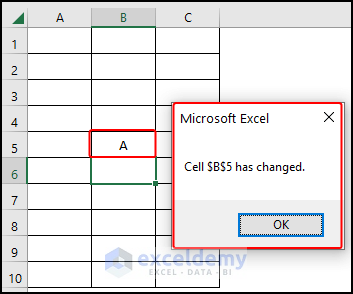
Thank you for your query. As far as I have understood your query, you want to change the copied values later and thus save it. Now, it is simple. You can do this normally. And, the values will be changed and saved automatically. But, to make this more effective and dynamic, you might need to have a confirmation window for this. To accomplish this, follow the steps below.
Steps:
Code:
Private Sub Worksheet_Change(ByVal Target As Range)Dim KeyCells As Range' The variable KeyCells contains the cells that will' cause an alert when they are changed.Set KeyCells = Range("A1:C10")If Not Application.Intersect(KeyCells, Range(Target.Address)) _Is Nothing Then' Display a message when one of the designated cells has been' changed.' Place your code here.MsgBox "Cell " & Target.Address & " has changed."End IfEnd SubThis code is taken from https://learn.microsoft.com/en-us/office/troubleshoot/excel/run-macro-cells-change
Now, if you insert any new value or remove any value from the cells A1:C10, there will be a Microsoft Excel window informing you about a change in the values. You can change this range inside the code as per your requirements.
I hope this accomplishes your desired result.
Regards,
Tanjim Reza
Hello, AHMED!
Thank you for your query. Regarding your query, you can use an array formula to accomplish this result.
Thus, all the cell values will be copied to all the desired cells in an instant.
I hope this solves your problem.
Regards,
Tanjim Reza
Hello, KASHIF!
Thank you for your query. Regarding your query, if you want to return value for meeting date condition only, you can use the INDEX-MATCH combination with the following formula.
=IFERROR(INDEX($E$5:$E$13,MATCH(H5,$D$5:$D$13,0)),"Not Available")If you want to meet the Product criteria and also the Date criteria, you can use the formula below.
=IFERROR(INDEX($E$5:$E$13,MATCH(1,(($B$5:$B$13=G5)*($D$5:$D$13=H5)),0)),"Not Available")I hope your problem is resolved now.
Regards,
Tanjim Reza
Hello, CRYSTAL!
Thank you for your query.
As far as I understood your question, you want to apply date criteria and multiple Category criteria in your formula to find the average of a different column.
You can accomplish this using the nested FILTER function along with the AVERAGE, EOMONTH, and DAY functions and you have to use the plus sign between the categories to enable the OR criteria. The final formula would look like this.
=AVERAGE((FILTER('ONLINE MASTER'!$D$2:$D$1000,(('ONLINE MASTER'!$F$2:$F$1000="COMPUTER")+('ONLINE MASTER'!$F$2:$F$1000="TELEPHONE"))*('ONLINE MASTER'!$A$2:$A$1000>=('2022'!$A63-DAY('2022'!$A63)+1))*('ONLINE MASTER'!$A$2:$A$1000<=EOMONTH(('2022'!$A63-DAY('2022'!$A63)+1),0)))))I hope this solves your problem.
With Regards,
Md. Tanjim Reza Tanim
Hey, YIANNIS ZOUGANELIS!
Thank you for your query. Hope you are doing well. You have asked some thoughtful questions. I am answering all your queries one by one below.
Q1: First of all, you have asked if it is possible to have the ENTER NEW DATA button on a different worksheet.
Yes, this is very much possible. In this regard, you will have to follow the same procedures of the article to create the forms and buttons for everything in the worksheet just where you want the button to appear.
Q2: Second, you want the selected worksheet not to become active. In this regard, you have to change the code a little bit. Say, you have set the button in the MainSheet worksheet. Now, you want to be active in this sheet all along. You don’t want to activate any other selected worksheet.
In this regard, create the button and form in the MainSheet worksheet and then write the code below inside the Code window of the Command_Button1.
Code:
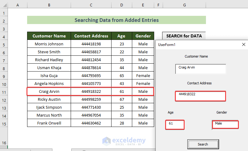
Private Sub CommandButton1_Click()TargetSheet = ListBox1.ValueIf TargetSheet = "" ThenExit SubEnd IfWorksheets(TargetSheet).ActivatelastRow = ActiveSheet.Cells(Rows.Count, 1).End(xlUp).RowActiveSheet.Cells(lastRow + 1, 2).Value = TextBox1.ValueActiveSheet.Cells(lastRow + 1, 3).Value = TextBox2.ValueActiveSheet.Cells(lastRow + 1, 4).Value = TextBox3.ValueActiveSheet.Cells(lastRow + 1, 5).Value = TextBox4.ValueWorksheets("MainSheet").ActivateEnd SubQ3: Thirdly, you want to search for present values rather than entering values. This is a different thing. Say, you are given the same dataset as per the article. Now, you want to enter only the customer’s name and want to get the contact address, age, and gender. Go through the steps below to achieve this.
Steps:
Sub Search_Data() UserForm1.Show End SubCode:
Sub SearchButton_Click()Dim sh As WorksheetSet sh = ThisWorkbook.Sheets("Search")Dim lr As Longlr = sh.Range("B" & Rows.Count).End(xlUp).RowDim i As LongIf Application.WorksheetFunction.CountIf(sh.Range("B:E"), Me.TextBox1.Text) = 0 ThenMsgBox "No match found!", vbOKOnly + vbInformationCall ResetExit SubEnd IfFor i = 2 To lrIf sh.Cells(i, "B").Value = Me.TextBox1.Text ThenTextBox1 = sh.Cells(i, "B").ValueTextBox2 = sh.Cells(i, "C").ValueTextBox3 = sh.Cells(i, "D").ValueTextBox4 = sh.Cells(i, "E").ValueEnd IfNext iEnd SubFunction Reset()TextBox1.Value = ""TextBox2.Value = ""TextBox3.Value = ""TextBox4.Value = ""End FunctionFinally, you will be able to get your desired automated search result.
Regards,
Tanjim Reza
Hello, PJ!
Hope you are doing well. Thank you for your query.
Cooling time mainly refers to the time elapsed from the end of holding pressure to the opening of the mold. This value depends on various factors like the wall thickness, product shape, mold temperature, melt properties, etc. To get a better product, the cooling time should be as low as possible.
You can search google thoroughly or visit industrial yards to learn about the actual cooling time values.
Regards,
Md. Tanjim Reza Tanim
Hello, NICK!
Hope you are doing well. Thank you for your query.
As we have used different functions in the two methods, the answer varied a little bit, it’s true. But as you can see, this variation is minimal. The final answer is almost equal in both methods. Moreover, the little variation is after the decimal part in a percentage format. So you can neglect this small difference most of the time to calculate the following approximate result.
But if you need a 100% accurate answer, I would suggest you use the manual method.
Regards,
Tanjim Reza
Hello, DJ!
Thank you for your query.
To analyze your problem, I would say it would be impossible to automate the sheet names completely without saving the file as an xlsm file.
As far as I understood you want to create as many sheets as you want and then extract values from them in other sheets automatically whenever you want. In this regard, you want to address the sheets automatically without writing their names in the formulas.
Now, In this process, VBA codes are the most appropriate to use. Without VBA codes, you have another way to do this by using the GET.WORKBOOK() function. But, you will need to save the file as an xlsm file even in this process. But, as your VBA is locked down, I am afraid you would not be able to work with xlsm file.
So, I would say this would be quite impossible to solve your problem with VBA locked down.
Regards,
Tanjim Reza
Hello, ADIL M!
Thank you for your appreciation and query.
Regarding your query, I have thought of two cases.
Case 1: Stacking all data in a single column but different rows with your desired order (A1, A2, B1, B2, and so on).
Case 2: Combining data of columns into separate cells, i.e. A1:A4 range in cell D1, B1:B4 range in cell D2, C1:C4 range in cell D3, and so on.
Download Link:
The file is attached here for you.
Solution.xlsx
⊕ 1st Case: Stacking All Data in a Single Column
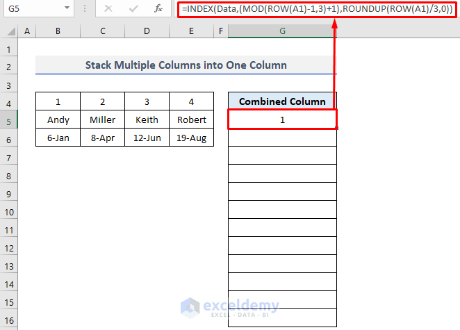
1. Use the following formula in cell G5.
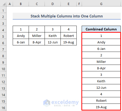
=INDEX(Data,(MOD(ROW(A1)-1,3)+1),ROUNDUP(ROW(A1)/3,0))2. Following, drag the fill handle downward to accomplish your full result.
Now, this formula may look like a complex one. So, for your better understanding, I am breaking down the formula below.
Formula Breakdown:
>> MOD(ROW(A1)-1,3)
This will give you the argument of the row number in the INDEX function. If you drag the fill handle it would give you the next row numbers as per your data range.
Result: 1,2,3,1,2,3,1,2,3,1,2,3 (As our range has 3 rows and 4 columns)
>> ROUNDUP(ROW(A1)/3,0)
This part will give you the sequence of column numbers for your data range. If you drag the fill handle below you would get all the column numbers individually for all the values of your range.
Result: 1,1,1,2,2,2,3,3,3,4,4,4
>> INDEX(Data,(MOD(ROW(A1)-1,3)+1),ROUNDUP(ROW(A1)/3,0))
This will take your lookup array and generate the values individually from the lookup as per the row numbers and column numbers that you have got in the upper processes. So after dragging the fill handle below, you will get the whole data range in a single column in your desired format.
Result: 1, Andy, 6-Jan, 2, Miller, 8-Apr, 3, Keith, 12-Jun, 4, Robert, 19-Aug
⊕ 2nd Case: Combining Data of Columns into Separate Cells
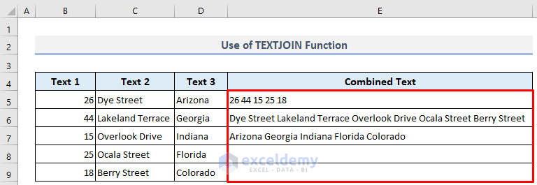
You can also use the TEXTJOIN function in this regard.
1. Insert the following formula in cell E5 now.
=TEXTJOIN(" ",TRUE,INDEX($B$5:$E$9,ROW($A$1),ROW(A1)):INDEX($B$5:$E$9,ROW($A$5),ROW(A1)))Note that the TEXTJOIN function can join an array of text. We have used the INDEX function as cell reference in the formula, to specify the array.
2. Following, drag the fill handle below to get all results.
Formula Breakdown:
>> INDEX($B$5:$E$9,ROW($A$1),ROW(A1))
This will return you the first row and first column data from your array. Here, you must reference your row_num argument with absolute reference.
Result: 26. 26 is situated in cell B5.
>> INDEX($B$5:$E$9,ROW($A$5),ROW(A1))
This will return you the last row of the following column data of your array.
Result: 18. 18 is situated in cell B9.
>> INDEX($B$5:$E$9,ROW($A$1),ROW(A1)):INDEX($B$5:$E$9,ROW($A$5),ROW(A1))
This refers to array B5:B9. To get this clearly, evaluate the formula from the Formulas tab.
>> TEXTJOIN(” “,TRUE,INDEX($B$5:$E$9,ROW($A$1),ROW(A1)):INDEX($B$5:$E$9,ROW($A$5),ROW(A1)))
This will join the texts from the first row to the last row of the first column of data with a space between each row of data.
Result: 26 44 15 25 18
Regards,
Tanjim Reza
Hello, John!

I hope you are doing well.
About your problem, I think your windows list separator is set to semicolon instead of comma. In this regard, follow the steps below to solve your problem.
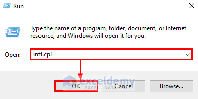
1. Go to your Windows menu and search for the Run window.
2. Afterward, open the Run window.
3. Now, write intl.cpl in the Open: text box.
4. Subsequently, click on the OK button.
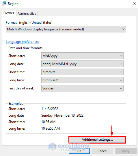
5. As a result, the Region window will appear.
6. Following, click on the Additional settings… button.
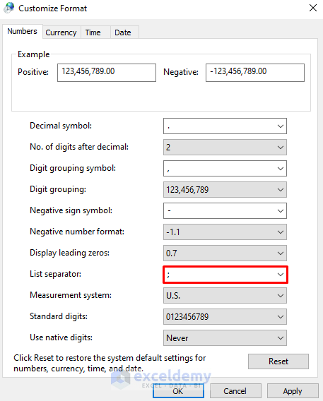
7. Consequently, the Customize Format window will appear. Here, you would see the List separator: option is selected as semicolon (;).
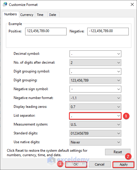
8. Following, change the List separator: option to comma (,) >> click on the Apply button >> click on the OK button.
9. Now close your Excel app and reopen the file. The formula will work fine.
Thus, I hope your problem would be solved now. If it doesn’t, please let us know in the comment section again.
Thanks,
Tanjim Reza
Hi Jay!
Thank you for your query!
Our formula here is correct.
Because, if you use
=IF(J3<>"",NOW(),"")in Cell K3, and copy it down column K, whenever you write something in column J, the NOW function will return the same timestamp in all cells of column K (K3, K4, K5,….). You will see no difference in the timestamps and will lose the original entry time.To fix this for each entry, you have to type
=IF(J3<>"",IF(K3="",NOW(),K3),"")in Cell K3, and copy it down the cells of column K. (You have to copy the formula first, even though there is no input in column J yet.)This formula is designed in such a way that the NOW function will not return the current time when there is already a timestamp recorded. Look closely,
IF(K3="",NOW(),K3)part ensures that the IF function will return what is already in column K cells if there is any priorly.Look at the following GIF image for more clarification.
Regards,
Tanjim Reza
Hi, MICHAEL V BERNOT!
Thank you for your query.
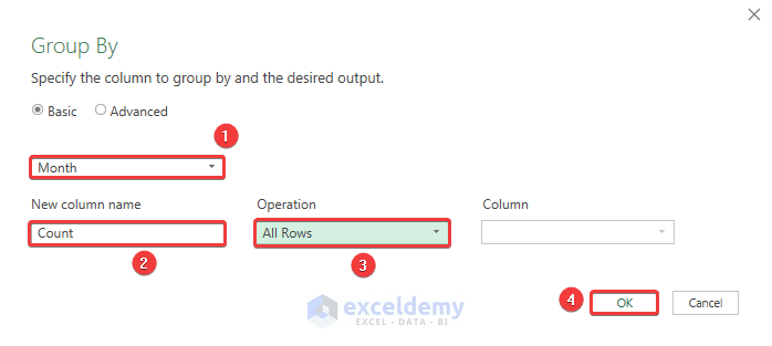
You have pointed out a good problem. To solve your problem remove the last bracket from the given Custom column formula in the article above.
And, another thing, choose the All Rows option in the Operation option list instead of Count Rows in the Group By window.
I hope this solves your problem. Stay with ExcelDemy for more Excel tips, tricks, formulas, and solutions.
Regards,
Tanjim Reza
Hi, Megan!
Thank you for your query.
You can definitely track change for multiple columns. If you want to track change for the A and B columns for row 5, then you can apply the following formula.
=IF(AND(A5="",B5=""),"",TODAY())Then you can use the fill handle feature for all the other rows.
Regards,
Tanjim Reza
Hi, Bill!
Thank you for your query.
Regarding your query, just make a dataset table and use the SUM function or the addition functionality of Excel. In our article, we have used the subtraction functionality; in your requirements, you just need to utilize the addition functionality of Excel.
Regards,
Tanjim Reza
Hi, GILBERT BECHTOL!
Thank you for your query.
In your appeared problem, I would suggest you use the MONTH function to get individual months from each date record. Then, sort the order from smallest to largest. As a result, you’ll get the billing months of the project in sequential order and thus you can use the INDEX function to achieve your target.
If your problem still doesn’t fix, please send us your Excel sheet with clearer feedback on your target in this regard.
Regards,
Tanjim Reza
Hi, BIJAN!
Thank you for your query.
You can achieve your desired result following the workflow below:
I hope, it helps.
Regards,
Tanjim Reza
Hi, KRISHNA!
Thank you for your query.
About your query, please check if you have put an equal sign (=) in the cell before inserting the formula. Because, on my end, your formula looks perfect. And, I checked it in my Excel sheet and it worked! If it still doesn’t work, please send us your excel file.
Regards,
Tanjim Reza
Hi, JAMAL!
You have pointed out the correct thing in response to BHANU’s problem.
Thank you for your valuable feedback!
Regards,
Tanjim Reza
Hi, BHANU!
Thank you for your query.
As the problem discussed here is sorted from smallest to largest, you would also need to sort your numbers before applying this article’s approach.
Regards,
Tanjim Reza
Hi, BHANU!
Thank you for your query.
As the problem discussed here is sorted from smallest to largest, you would also need to sort your numbers before applying this article’s approach.
Regards,
Tanjim Reza
Hi, JEFF!
Thank you for your query.
I am afraid you can not incorporate this article’s formula into the SUMIFS formula to perform a loop because we have used the MAX function in this article. But, it is a limitation of Excel to use the SUMIFS function with the MAX function.
To know about some other Excel limitations, you can follow the link below:
22 Limitations of Excel That Might Frustrate You
Regards,
Tanjim Reza
Hi, BANDEET POUDEL!
Thank you for your query.
I am a little bit confused about your query. Are you asking if you can jump to a row upon writing the row number at an instant?
If you are asking this, then the solution is:
You can write the preferred cell’s reference number in the name box and press the Enter button to jump there in an instant.
Please let us know the feedback if your problem is solved or if you meant some other things in your query.
Regards,
Tanjim Reza
Hi, VIJAY!
Thank you for your feedback!
Thank you for your appreciation, JUSTIN!
Thank you for your appreciation, FERREIRA!
Hi, WILL!
Thank you for your query!
You can definitely point to a cell containing the desired date rather than typing it inside the formula. Say, you have placed the required date in the C15 cell.
In that case, you can use the following formula:
Hello, KANHAIYALAL NEWASKAR!
Thank you so much for your appreciation.
We also hope to learn and share more and more knowledge with everyone!
Regards,
Tanjim Reza
Hi, ARUN!
Thank you for your query.
According to our dataset, we have 9 values that are repeated twice or thrice. Other values are unique and have come only once in the dataset. As the formula is about finding the frequent numbers, it is returning those repeated 9 numbers only.
Regards,
Tanjim Reza
Hi, GEOFF BARTLETT! We appreciate your thoughtful query.
Workaround 1:
For your first problem (Surname, forename2 forename1), you can use the formula below:
=SUBSTITUTE((RIGHT($B7,LEN($B7)-FIND("^",SUBSTITUTE($B7," ","^",LEN($B7)-LEN(SUBSTITUTE($B7," ",""))))))&" "&(MID($B7,SEARCH(" ",$B7)+1,SEARCH(" ",$B7,SEARCH(" ",$B7)+1)-(SEARCH(" ",$B7)+1)))&" "&(LEFT($B7,SEARCH(" ",$B7)-1)),",", "")And, for your second problem (Surname, forename2 forename3 forename1) you can use the formula below:
=SUBSTITUTE((RIGHT($B5,LEN($B5)-FIND("^",SUBSTITUTE($B5," ","^",LEN($B5)-LEN(SUBSTITUTE($B5," ",""))))))&" "&(MID($B5,SEARCH(" ",$B5)+1,SEARCH(" ",$B5,SEARCH(" ",$B5)+1)-(SEARCH(" ",$B5)+1)))&" "&"("&(MID($B5,SEARCH(" ",$B5,SEARCH(" ",$B5,1)+1)+1,SEARCH(" ",$B5,SEARCH(" ",$B5,SEARCH(" ",$B5,1)+1)+1)-(SEARCH(" ",$B5,SEARCH(" ",$B5,1)+1)+1)))&")"&" "&(LEFT($B5,SEARCH(" ",$B5)-1)),",", "")Workaround 2:
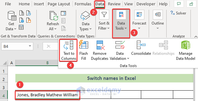
Besides, another workflow you can use in this regard. That is:
Step 1: Use the Text to Columns tool from the Data tab for splitting every name.
https://www.exceldemy.com/text-to-columns-excel/
Step 2: Sort them according to your desired sequence. Use a helper row for that. Use and finally >>
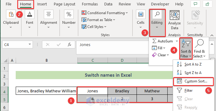
Last Step: Use the CONCATENATE function to combine them in a cell.
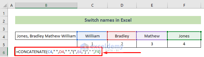
https://www.exceldemy.com/excel-concatenate-function/
Regards,
Tanjim Reza
Hi, JUSTIN!
Thank you for your query.
You can accomplish your desired result by using the formula below:
Regards,
Tanjim Reza
Hi, A!
Thank you for your query.
The FV formula that you need for your solution will be like this:
=FV([(Interest Rate-Inflation Rate)/Frequency of Payment Per Year],[Frequency of Payment Per Year * Total Years],[-Payment Per Period], Present Value,0)So, with your given values, the formula would be:
=FV(3%,41,-1000,0,0)Regards,
Tanjim Reza
Hi, ADRIAAN!
Thank you for your query.
The FV formula that you need for your solution will be like this:
=FV([(Interest Rate-Inflation Rate)/Frequency of Payment Per Year],[Frequency of Payment Per Year * Total Years],[-Payment Per Period], Present Value,0)So, with your given values, the formula would be:
=FV(3%,41,-1000,0,0)Regards,
Tanjim Reza
Hi, ERIC!
Thank you for your valuable feedback.
You have pointed out a nice thing. When the #VALUE! error happens in this regard, it is better to use the find and replace feature to replace ” ” with CHAR(160) before applying the formula.
Regards,
Tanjim Reza
Hi, JO JONES!
Thank you for your query.
Can you please tell me what you meant by the multiple strawberries in the criteria range? Does it mean that you are putting multiple strawberry categories in the range? If yes, then I would suggest you put the full name of the strawberries along with their categories in the cells. As a result, every strawberry name will be unique as per dates. Moreover, if a category has multiple data at multiple dates, then you can look up your value through the unique dates.
If your problem still exists, please let us know your feedback and help us understand your question better.
Regards,
Tanjim Reza
Hi, BRENT!
You have asked a fantastic question.
You can change the fill/text color automatically by using conditional formatting. You can apply multiple rules to a cell using this. To learn about conditional formatting in this regard, you can go to the following link.
https://www.exceldemy.com/excel-conditional-formatting-greater-than-another-cell/
Regards,
Tanjim Reza
Hello, KEITH FROST!
Thank you for your query.
There is no error in your code. You just need to add “filename:=filename” at the ActiveSheet.ExportAsFixedFormat command.
So, just write the export format command line as:
Regards,
Tanjim Reza
Hi, PAOLO!
Thank you for your query.
You have asked about a fantastic thing. If we want to compare the first 6 numbers/match, rather than the full cell value, we have to use the LEFT function in addition to the formulas.
So, I would suggest you use the second and third methods shown in this article and use the nested LEFT function inside the VLOOKUP function for the 2nd method and inside the MATCH function for the 3rd method.
So, for the second method, the formula would be:
=IF(ISNA(VLOOKUP(LEFT(A2,4),LEFT($B$2:$B$8,4),1,FALSE)),"NO","YES")And, for the third method, the formula would be:
=IF((ISERROR(MATCH(LEFT(A2,4),LEFT($B$2:$B$8,4),0))),A2,"")Have a nice day!
Hi, LAURA!
Thank you for your query.
Your query’s solution is very easy, but a little bit tricky. For the solution, at the name box of a cell, write the cell references of your desired cells where you want to put the same value by copying.
Let, you want to put the number 10 to B2:B160002 cells. Now, write B2:B160002 in the name box. As a result, your desired 160000 cells will be selected. Now, write 10 and press Ctrl + Shift + Enter.
Moreover, you can follow one of our articles named “How to Copy and Paste Thousands of Rows in Excel” to know more. The link to this article is given below.
https://www.exceldemy.com/how-to-copy-and-paste-thousands-of-rows-in-excel/
Have a nice day!
Hi, AHMAD AKAR!
Thank you for your query.
You have encountered an interesting problem. Regarding your query, we have a different article already posted on our website. Please follow the link below to learn about the solution to your query.
https://www.exceldemy.com/copy-and-paste-in-excel-when-filter-is-on/
Have a good day!
Hi, BELLA!
Thank you for your appreciation!
Hello, MARK EVANS!
You have pointed out a fantastic thing.
Your reference is correct. We had an unfortunate mistake in the reference to this formula. There will be L8 at the reference in the place of the C10 reference.
Thank you for your valuable feedback. We appreciate it so much.
So, the formula should be:
=SUMPRODUCT(D5:I14,(C5:C14=L8)*(D4:I4=L9)*(B5:B14=L7))Regards,
Tanjim Reza
Hi PAUL R HARTLEY! Thank you for your query.
You can fix these links easily using the following process.
Go to the Data tab >> Queries & Connections group >> Edit Links tool.
Afterward, all the links used in this workbook will be shown to you in the Edit Links window. Select individual links and click on the Check Status button for each of them.
If you see an Error: Source not found in any status, click on the Change Source button. Subsequently, browse your “form” Excel sheet >> click on the OK button >> click on the Close button of the Edit Links window.
Regards,
Tanjim Reza
Hello, W BREKVELD!
Thank you for your query.
Yes, you can multiply a value with the looked-up percentage corresponding with a year. Just use the VLOOKUP function properly. Then write your desired multiplier in the formula bar before the used VLOOKUP function and then insert an asterisk (*) symbol.
Thus, the value will be multiplied by the looked-up percentage. And, to do this until the current year, use your fill handle feature to copy the same formula.
Regards,
Tanjim Reza
Hello, TEMITOPE!
You have asked a nice thing. Using VLOOKUP with dates is a complex thing sometimes and may result in errors easily. In this regard, you need to use the TEXT function.
Suppose, you have 5 columns in your table. You want the fifth column value for the C16 text and C15 date value. The date column is in the C5:C13 cells. In this situation, you can use the following formula for using VLOOKUP with text and date.
=VLOOKUP(C16,IF(TEXT(C5:C13,"mm/dd/yy")=TEXT(C15,"mm/dd/yy"), B5:F13, ""), 5, FALSE)Thank you for your query. We appreciate it so much.
Regards,
Tanjim Reza
Hello, NIEFER!
You have pointed out a fantastic thing.
It is correct that you don’t need to merge the cells B:D here. You can just enlarge the B column as much as you need. I just wanted to keep the column size closer to each other. That’s why I merged. But, it is not necessary. Rather, it is better to enlarge the B column as the references will be simpler that way.
Thank you NIEFER for your valuable feedback. I appreciate it so much.
Regards,
Tanjim Reza