Method 1 – Using CONCATENATE Function with Texts
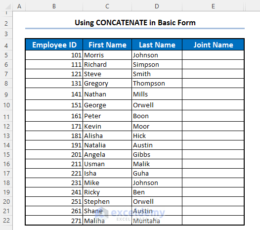
The sample dataset has Employee IDs, First Names, and Last Names in different columns. We will concatenate the first names and the last names.
- Add the formula below in cell E5 and press enter.
=CONCATENATE(C5,D5)
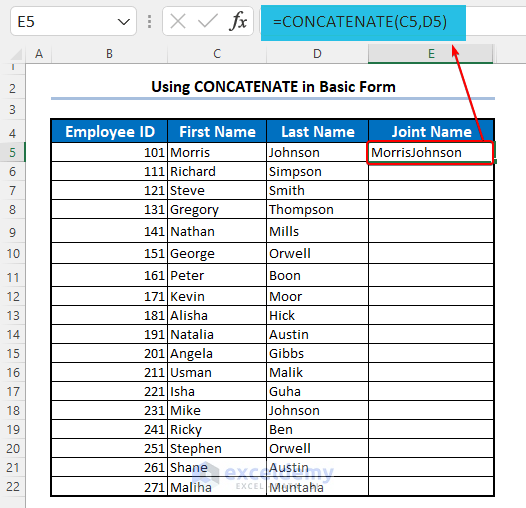
- There is no space between the first and last names, so you need to insert a space in between.
- The space itself is a text value. Concatenate the space with the names using this formula:
=CONCATENATE(C5," ",D5)
This formula concatenates the text values of the cells C5, D5, and a space “ ” into one single text.
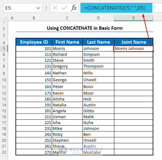
- The name will display correctly.
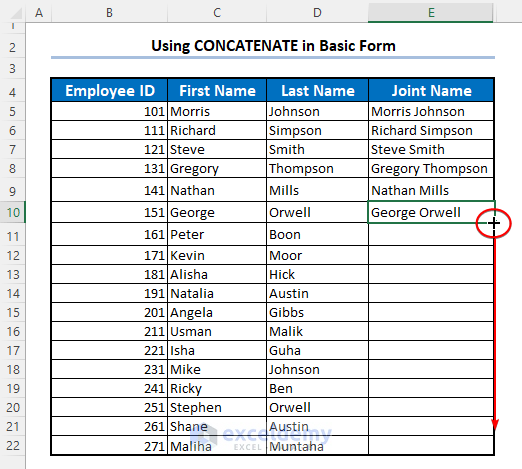
- Drag or double-click on the Fill Handle to copy the formula for the rest of the employees.
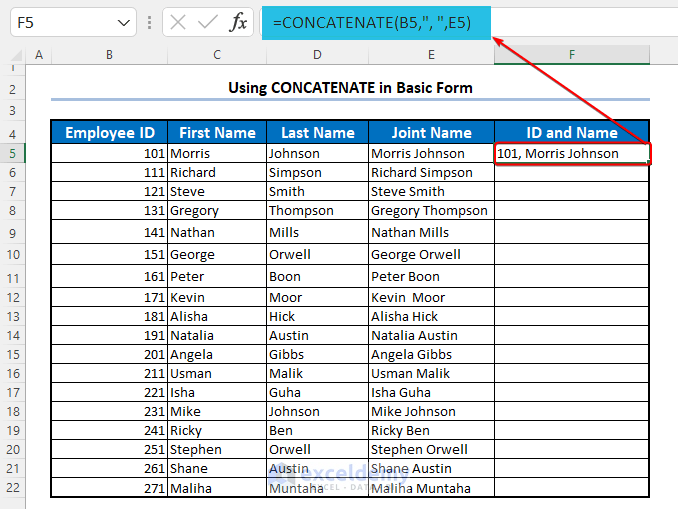
Method 2 – Using CONCATENATE Function with Numbers
To join the Employee IDs and the names into a single cell,
- Apply the following formula in cell F5.
=CONCATENATE(B5,", ",E5)
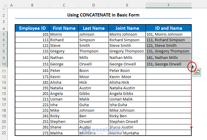
This formula joins the number in cell B5, a comma with a space, and the text value in cell E5 into one single text.
- Drag the Fill Handle to copy the formula to the rest of the cells.
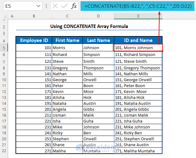
Method 3 – Using CONCATENATE Function for Ranges
- CONCATENATE function cannot recognize an array, i.e. if you want to join values in cells A1, A2, A3, and A4, you cannot write the argument as (A1:A4), rather it must be (A1,A2,A3,A4). You have to separate the inputs with commas in the function.
- But you can separate arrays as arguments.
To concatenate the IDs, First Names, and Last Names of all the employees into one single cell using an Array Formula,
- Select all the cells together and enter this Array Formula in the first cell:
=CONCATENATE(B5:B22,", ",C5:C22," ",D5:D22)
- Press Ctrl + Shift + Enter. (or just press Enter if you are using Excel 365)
Formula Breakdown:
If we break the Array Formula, we will get 18 single formulas like this:
- CONCATENATE(B5,”, “,C5,” “,D5)
- CONCATENATE(B6,”, “,C6,” “,D6)
- CONCATENATE(B7,”, “,C7,” “,D7)
…
…
…
- CONCATENATE(B22,”, “,C22,” “,D22)
CONCATENATE(B5,”, “,C5,” “,D5) joins the number in cell B5, a comma with a space, the text in cell C5, another space, and the text in cell D5 together.
Method 4 – Using CONCATENATE Function to MATCH Multiple Criteria Equal to a Value
The sample dataset contains marks of students in Physics, Chemistry, and Biology, and we want to find out the student who got 100 in all three subjects.
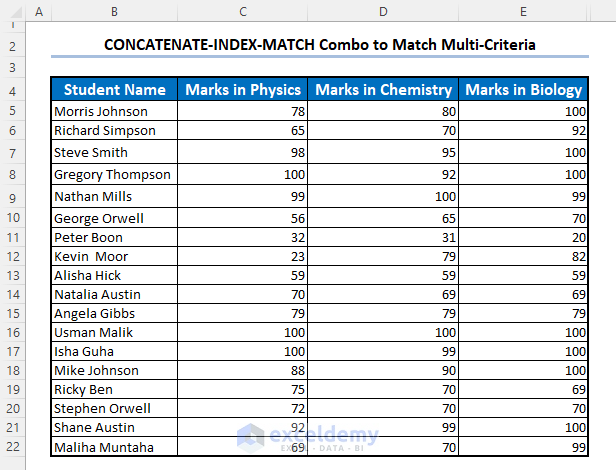
- Apply the formula below in cell F5.
=INDEX(B5:E22,MATCH("100100100",CONCATENATE(C5:C22,D5:D22,E5:E22),0),1)
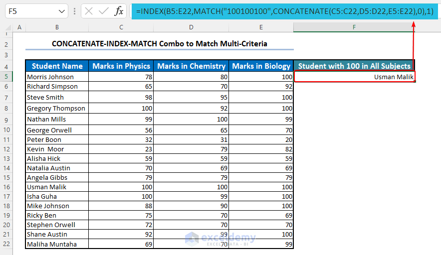
It will output the name of the student who scored 100 in all three subjects, Usman Malik.
Formula Breakdown:
- CONCATENATE(C5:C22,D5:D22,E5:E22) joins all values of the arrays C5:C22, D5:D22 and E5:E22 into single text values.
For the first student, it joins 78, 80, and 100 and returns “7880100”.
For the student with 100 in all 3 subjects, it returns “100100100”. - MATCH(“100100100”,CONCATENATE(C5:C22,D5:D22,E5:E22),0) returns the row number in the table where marks in all three subjects are 100.
- INDEX(B5:E22,MATCH(“100100100”,CONCATENATE(C5:C22,D5:D22,E5:E22),0),1) returns the value in the cell with row number equal to the output of the MATCH function and column number equal to 1 from the table array B5:E22.
The student who got 100 in all three subjects is Usman Malik.
Note:
- It is an Array Formula, so you must press Ctrl + Shift + Enter to insert this formula.
- This method only works for cases where the criteria are equal to some values. If the criteria are greater than or less than some values, this method will not work. For example, you can not identify the student who got greater than 95 in all subjects in this way.
- If more than one value satisfies all the criteria, you will get only the first value in this process. To get all the values that satisfy all the criteria, use the FILTER function instead.
Common Errors with CONCATENATE Function of MS Excel
| Error | When They Show |
|---|---|
| #N/A! | This shows when the arguments are arrays instead of single values, and the lengths of all the arrays are not the same. |
| #VALUE! | This shows when the arguments are invalid. |
| #NAME? | This shows when quotation marks are missing for Text arguments. |
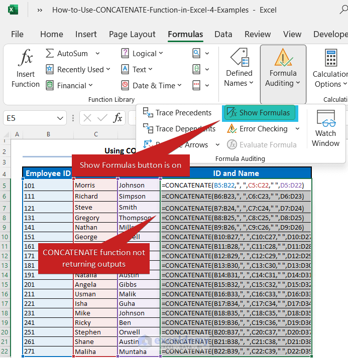
Some More Reasons for Excel CONCATENATE Not Working:
-
- Check if the Show Formulas option is on in the Formula Auditing section of the Formulas tab.
-
- If you pass the inputs as range, the function will not work. You can try the CONCAT function for this.
Download Practice Workbook
<< Go Back to Excel Functions | Learn Excel
Get FREE Advanced Excel Exercises with Solutions!Rifat Hassan, BSc, Electrical and Electronic Engineering, Bangladesh University of Engineering and Technology, has worked with the ExcelDemy project for almost 2 years. Within these 2 years, he has written over 250 articles. He has also conducted a few Boot Camp sessions on effective coding, especially Visual Basic for Applications (VBA). Currently, he is working as a Software Developer to develop and deploy additional add-ins to enhance the customers with a more sophisticated experience with Microsoft Office Suits,... Read Full Bio


please send me the full text book on this .
Dear Ronhat Minmin,
If you want to get the Excel File, you can download it from Download Practice Workbook
Regards
ExcelDemy