Here’s an overview of highlighting cells if they have higher values than other cells in a range.
Highlight a Cell If Its Value Is Greater Than Another Cell in Excel: 6 Ways
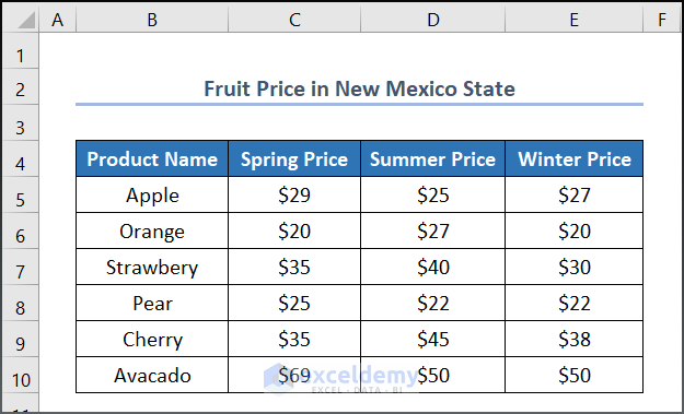
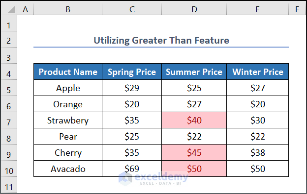
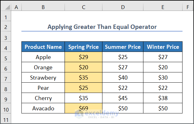
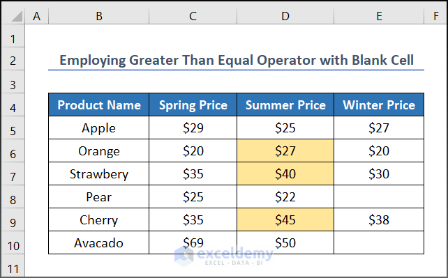
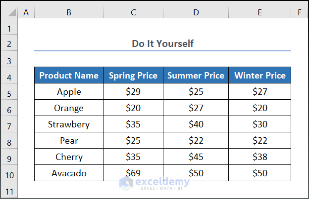
Consider the following dataset, which contains 4 columns that represent fruit prices in different seasons. We will show the season where prices are higher.
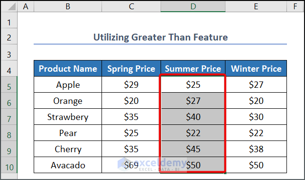
Method 1 – Utilizing the Greater Than Feature to Highlight a Cell If Its Value Is Greater Than Another Cell
Steps:
- Select the cell or cell range. We selected the cell range D5:D10.
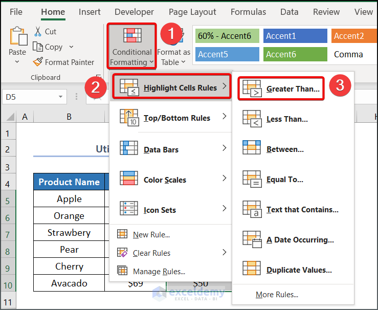
- Go to the Home tab and select Conditional Formatting.
- Under Highlight Cells Rules, select Greater Than.
- A dialog box will pop up.
- In Format cells that are GREATER THAN, select the other cell with which you want to compare. Let’s select the E5 cell.
- Select any format to color where values are Greater Than. We selected Light Red Fill with Dark Red Text.
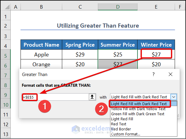
- Click OK. This will highlight all cells that have higher value than that singular cell.
Read more: Conditional Formatting Based On Another Cell in Excel
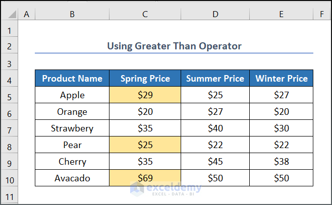
Method 2 – Using the Greater Than (>) Operator to Highlight a Cell If Its Value Is Greater Than Another Cell
Steps:
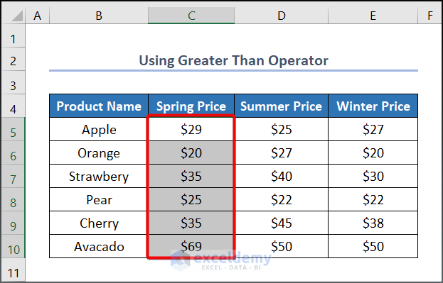
- Select the cell or cell range. We selected the cell range C5:C10.
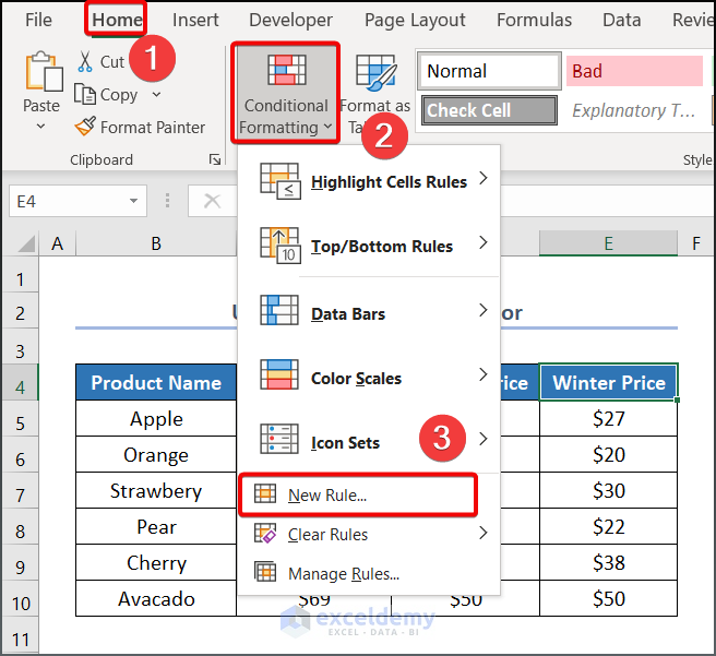
- Open the Home tab and go to Conditional Formatting.
- Select New Rule.

- A dialog box will pop up.
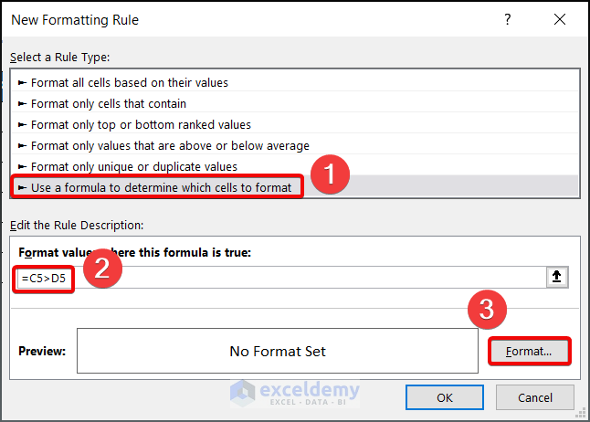
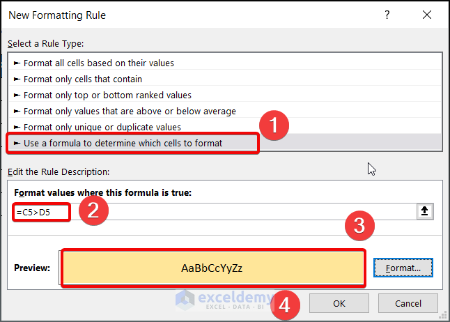
- From Select a Rule Type, choose Use a formula to determine which cells to format.
- In Format values where this formula is true insert the following formula.
=C5>D5- Click on Format.
- A dialog box will pop up.
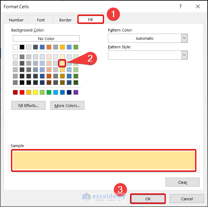
- Select a color in the Fill tab and press OK.
- Click OK.
- This will highlight the cell values of the Spring Price column where a cell is greater than the corresponding value in the Summer Price column.
Read more: Excel Conditional Formatting Based on Multiple Values of Another Cell
Method 3 – Applying the Greater Than Equal (>=) Operator to Highlight a Cell If Its Value Is Greater Than Another Cell
Steps:
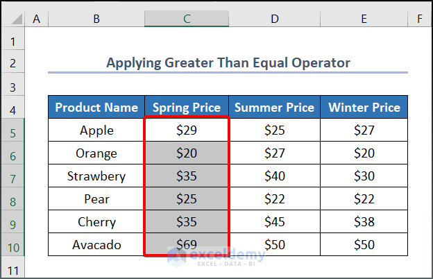
- Select a cell or cell range you want to highlight. We selected the cell range C5:C10.
- Go to Conditional Formatting and select New Rule
- A dialog box will pop up.
- From Select a Rule Type, choose Use a formula to determine which cells to format.
- In Format values where this formula is true, insert the following formula.
=C5>=E5- From Format, select the format of your choice.
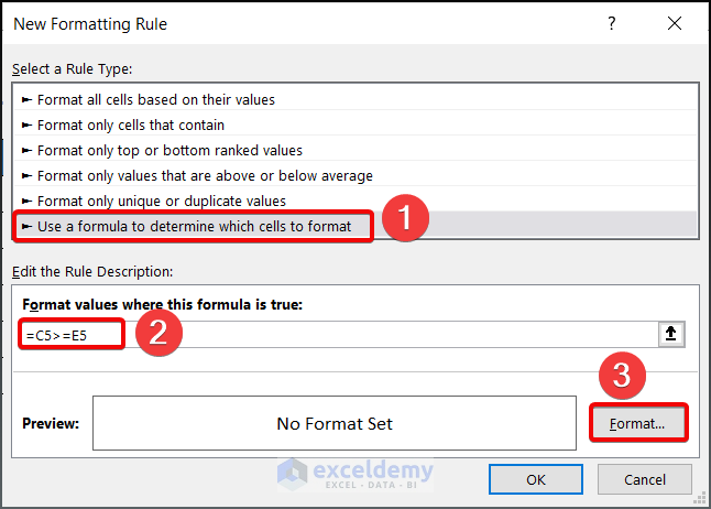
- Click OK. This highlights values if they are higher than in the Winter Price column.
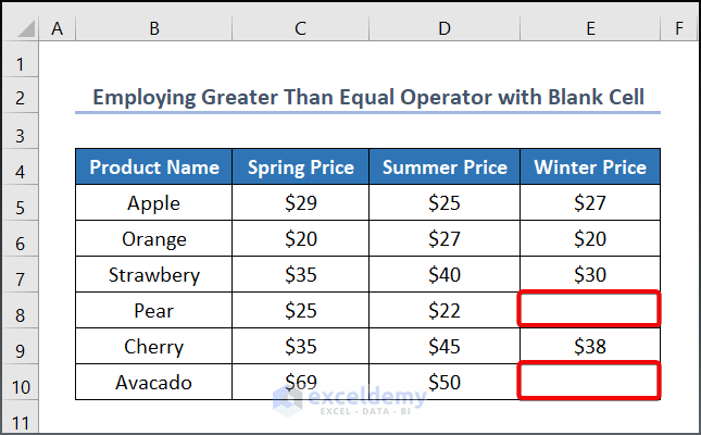
Method 4 – Using Greater Than Equal (>=) with Blank Cells to Highlight a Cell If Its Value Is Greater Than Another Cell
We put some blank cells that we’ll need to skip.
Steps:
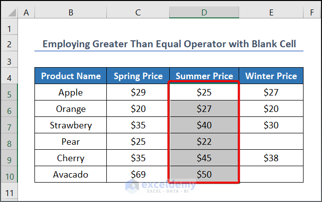
- Select a cell or cell range. We selected the cell range D5:D10
- Go to Conditional Formatting and select New Rule

- A dialog box will pop up.
- Select Use a formula to determine which cells to format.
- Insert the following formula.
=AND(D5>E5, $E5<>"")
- Select the format of your choice in Format.
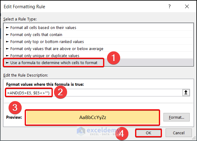
- Click OK. This compares the values between cells in the Summer Price and Winter Price columns, but only if the latter values are not empty.
Read more: Conditional Formatting for Blank Cells in Excel
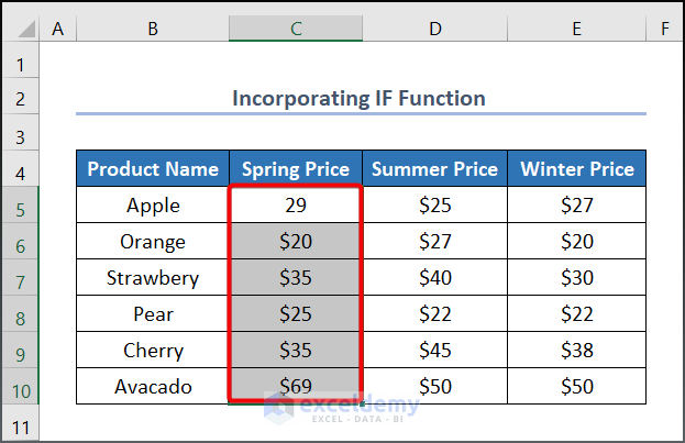
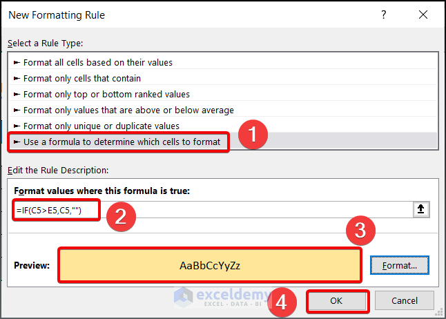
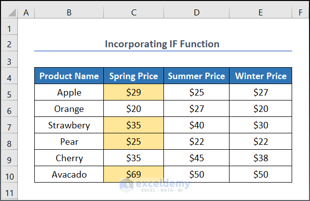
Method 5 – Incorporating the IF Function to Highlight a Cell If Its Value Is Greater Than Another Cell
Steps:
- Select a cell or cell range. We selected the cell range C5:C10
- Go to Conditional Formatting and select New Rule.

- Adialog box will pop up.
- Pick Use a formula to determine which cells to format.
- In Format values where this formula is true, insert the following formula.
=IF(C5>E5,C5,"")=IF(C5>E5,C5,””) checks that cell C5 is greater than E5. If the selected cell is greater than E5 then, it will highlight the C5 cell.
- From Format, select the format of your choice to highlight the cell.
- Click OK.
Read more: Excel Conditional Formatting Formula with IF
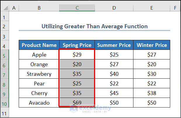
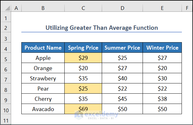
Method 6 – Utilizing the Average Function to Highlight Cells Based on Greater Average Value
We’ll calculate the average of the Summer Price and the Winter Price columns and check whether cells in the Spring Price column have a higher value than the average.
Steps:
- Select the cell range C5:C10.
- Go to Conditional Formatting and select New Rule.

- A dialog box will pop up.
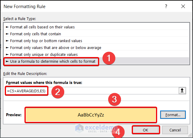
- Pick Use a formula to determine which cells to format.
- In Format values where this formula is true, insert the following formula:
=C4>AVERAGE(D4,E4)
C4>AVERAGE(D4,E4) calculates the average of the value from D5 and E5, and then we are checking whether the C5 value is greater than the derived value or not.
- From Format, select the format of your choice.
- Click OK.
Practice Section
We’ve provided a practice sheet to practice the explained methods.
Download to Practice
Further Readings
- How to Format Cell Based on Formula in Excel
- How to Use Conditional Formatting Based on VLOOKUP in Excel
- How to Apply Conditional Formatting with INDEX-MATCH in Excel
- Excel Conditional Formatting Formula If Cell Contains Text
- Applying Conditional Formatting for Multiple Conditions in Excel
- Conditional Formatting If Cell is Not Blank
- How to Change Text Color Based on Value with Excel Formula
- Conditional Formatting Multiple Text Values in Excel
- Conditional Formatting Entire Column Based on Another Column in Excel
<< Go Back to Conditional Formatting with Multiple Conditions | Conditional Formatting | Learn Excel
Get FREE Advanced Excel Exercises with Solutions!

Shamima thank you
I was hoping to make a rule where a row of new inputs are made green color if they are greater than the previous row. The rule creation doesn’t seem to let me pick more than one cell at a time.
Hello John,
You’re welcome! You can apply conditional formatting to an entire row by using a formula. Select the entire range of rows where you want the rule to apply, then use a formula like
=A2>A1 (adjust for your specific columns). This way, the whole row will turn green if the new values are greater than the previous row. Let me know if you need more details!
Regards
ExcelDemy