Conditional Formatting Entire Column Based on Another Column in Excel

In Excel, conditional formatting is used to highlight any cells based on predetermined criteria and the value of those cells. We can also apply conditional formatting to highlight an entire column based on another column. In this article, you will get to know how you can apply conditional formatting entire column based on another column in Excel with some easy easy steps.

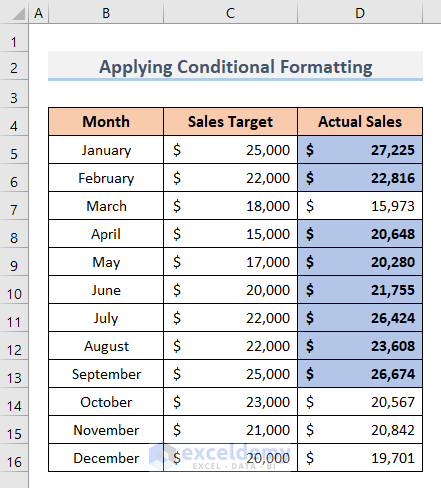
Let’s say we have a Sales Report for the year 2022 of a company. Every month there was a Sales Target. Now we will use conditional formatting to find out the Actual Sales which were higher than the Sales Target.

Step 1: Select Single Column to Apply Rules

To apply Conditional Formatting first you have to select the cells. If you want to highlight the entire row after applying conditional formatting, you need to select all of your datasets. But to highlight cells from a single column you just need to select the cells of that column.

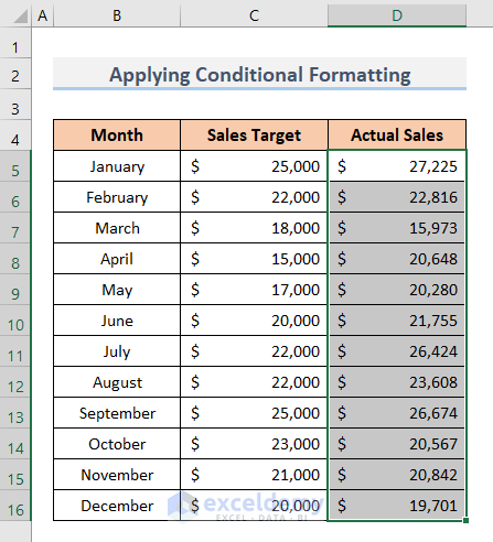
For our dataset, we want to apply conditional formatting to Column D. So, we have selected the cells of Column D only.

Read More: Excel Conditional Formatting on Multiple Columns

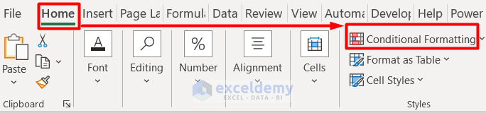
Step 2: Open New Format Rule Window from Conditional Formatting

In the second step, you need to open the New Format Rule window from the Conditional Formatting panel to choose suitable formatting rules according to your need.

• First, go to the Home tab and click on Conditional Formatting to expand it.

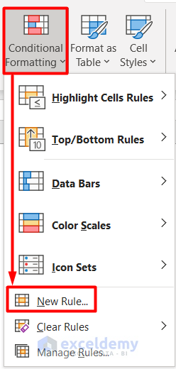
• Now, you will see different rules for applying conditional formatting. You need to choose a rule based on your criteria.
• therefore, to apply conditional formatting in a column based on another column, we need to select New Rule.

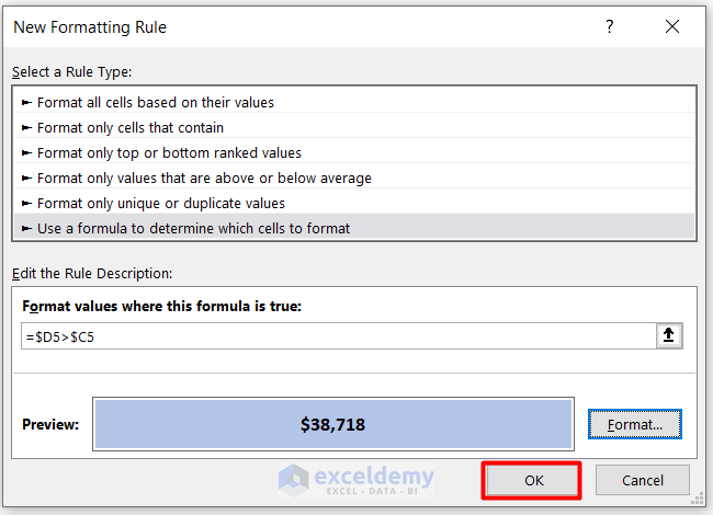
• After that, a window named New Formatting Rule will appear.
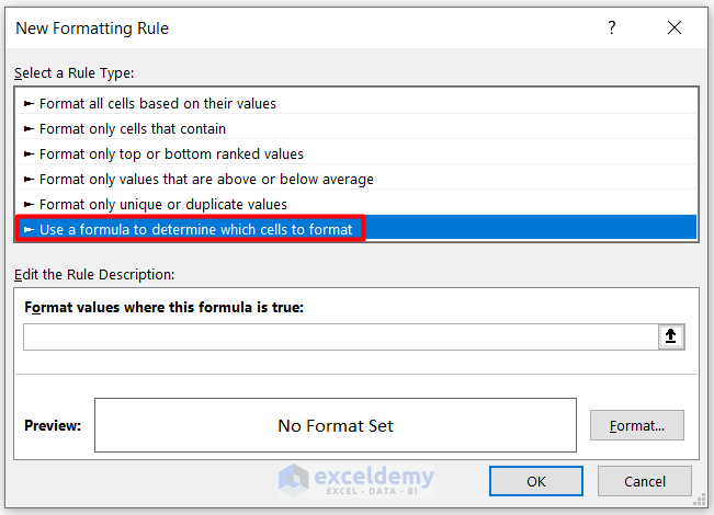
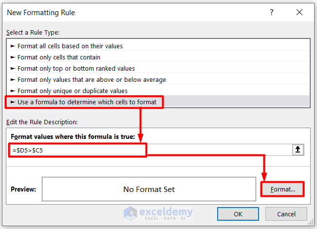
• Here, select Use a formula to determine which cells to format from the Select a Rule Type Box.

Read More: Applying Conditional Formatting for Multiple Conditions in Excel

Step 3: Insert Formula for Conditional Formatting

After selecting Use a formula to determine which cells to format a box named Format values where this formula is true will appear below the Select a Rule Type box.

• Here, type the following formula in the box.

• After that, you need to fix the formatting style, and to do that click on the Format box.

Read More: How to Use Conditional Formatting in Excel

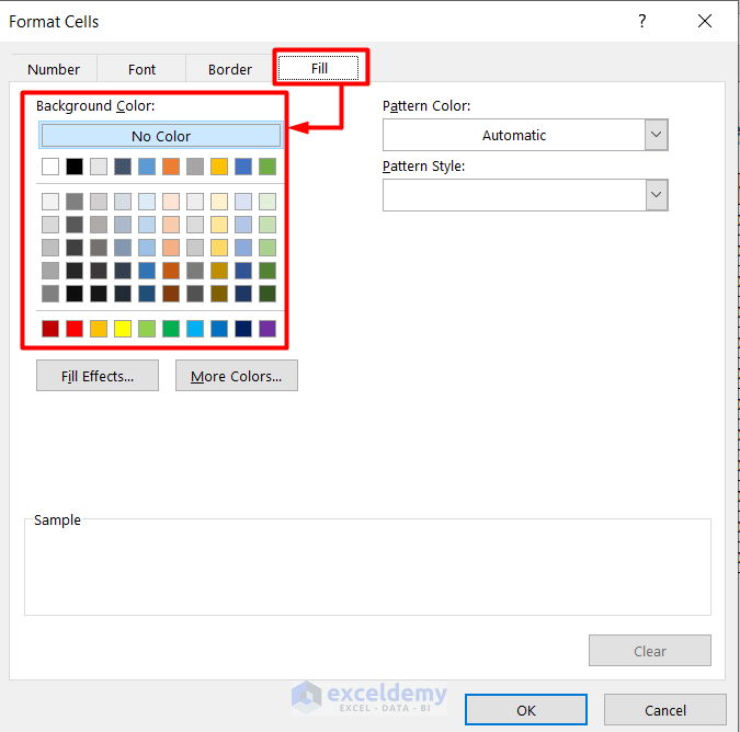
Step 4: Determine Formatting Style

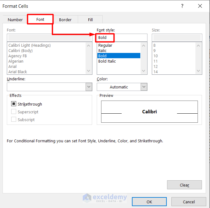
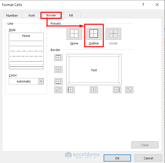
After clicking on the Format box a new window named Format Cells will appear. Here you can choose different formatting styles from different tabs of the window.

• First, from the Number tab, you can choose different numbering formats for the formatted cells.
• As we have sales data in our dataset, we have chosen Accounting.

• Then, from the Font tab select Bold as the font style. So after applying conditional formatting we will get bold fonts in the formatted cells.

• Afterward, from the Border tab, you can choose different styles for the border of the formatted cells. We have chosen Outline Presets in our example.

• Finally, from the Fill tab, you can choose your preferred Background Color.
• Also, feel free to select the Pattern Color, Pattern Style, and Fill Effects for conditional formatting.
• At last, after setting your preferred formatting style click on OK.

Step 5: Apply Conditional Formatting to Selected Column Based on Another Column

You are all set to apply conditional formatting to an entire column based on another column.

• After Step 4, you will see your selected formatting style in the Preview box in the New Formatting Rule window.
• Now, click OK to apply conditional formatting in your selected column.

• Finally, after pressing OK, you will see conditional formatting is applied to your selected Column D based on Column C.

Additional Tips

• If you want to apply Conditional Formatting to more cells of the same column in the future, then initially select some additional cells,(for example, up to 100 rows) and then go through the steps above.
• Otherwise, you can convert the dataset into a Table (Insert > Table) including additional rows. After that, apply Conditional Formatting to the selective column and it will work automatically for future inserts.

Things to Remember

• Make sure you only refer to the columns as Absolute Cell References, not the row numbers.
• Always refer to the top left cell of the selected column where the values start.
• If you copy the rule with Format Painter from one column to another, make sure to check on the column reference.

Download Practice Workbook

Download this sample file to practice by yourself.

Conclusion

This article gives you the basic guidelines for conditional formatting an entire column based on another column in Excel. So if you follow the steps described in this article you will be able to apply conditional formatting to columns based on the criteria from other columns. Feel free to leave a comment, if you have any confusion.

Related Articles

• How to Format Cell Based on Formula in Excel
• How to Use Conditional Formatting Based on VLOOKUP in Excel
• How to Apply Conditional Formatting with INDEX-MATCH in Excel
• Excel Conditional Formatting Formula with IF
• Excel Conditional Formatting Formula If Cell Contains Text
  
• Conditional Formatting If Cell is Not Blank
• How to Change Text Color Based on Value with Excel Formula
• Conditional Formatting Multiple Text Values in Excel
  
• Excel Highlight Cell If Value Greater Than Another Cell

<< Go Back to Conditional Formatting with Multiple Conditions | Conditional Formatting | Learn Excel