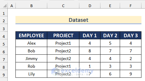
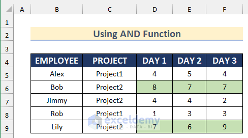
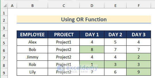
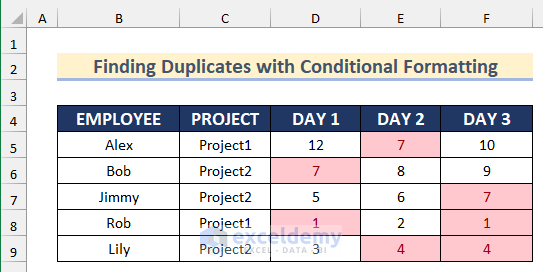
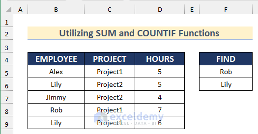
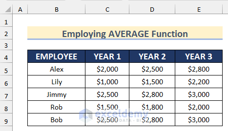
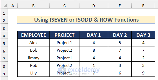
The sample dataset (B4:F9) contains names of employees, their projects and their working hours on different days.
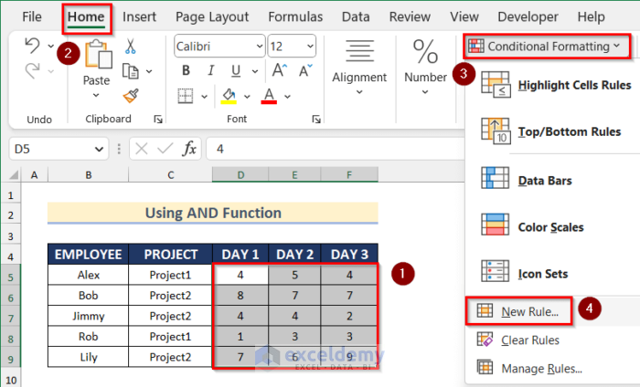
Method 1 – Use the AND Function with Conditional Formatting on Multiple Columns
STEPS:
- Select the range D5:F9 (working hours).
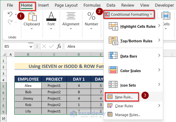
- Go to the Home tab.
- Select Conditional Formatting >> New Rule.
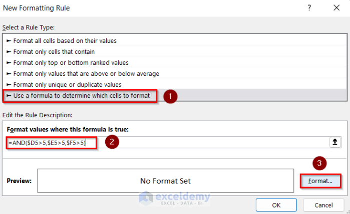
- The New Formatting Rule window will open.
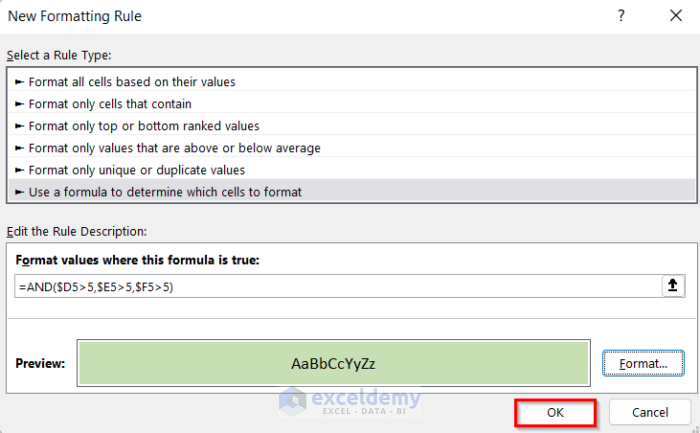
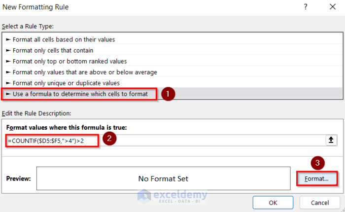
- After that, go to Use a formula to determine which cells to format.
- Enter the following formula.
=AND($D5>5,$E5>5,$F5>5)- Select Format.
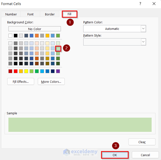
- In Format Cells, go to the Fill tab.
- Select a background color.
- Sample shows the color preview.
- Click OK.
- Click OK again.
This is the result.
Formula Breakdown
The AND function will return TRUE if D5, E5, F5 are greater than 5; otherwise FALSE. Conditional Formatting will apply the formula to the whole dataset.
Read more: Applying Conditional Formatting for Multiple Conditions in Excel
Method 2. Applying Conditional Formatting on Multiple Columns with the OR Function in Excel
STEPS:
- Open New Formatting Rule (as shown in Method 1).
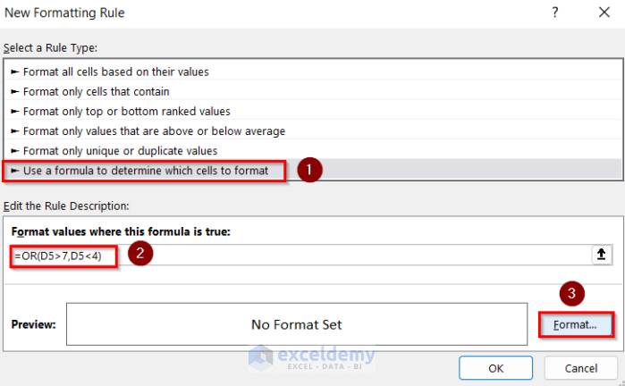
- Go to Use a formula to determine which cells to format.
- Enter the following formula.
=OR(D5>7,D5<4)- Go to Format and select the cell background color.
- Click OK.
This is the output.
Formula Breakdown
The OR function will return TRUE if D5 is greater than 7 or less than 4; otherwise FALSE. Conditional Formatting will apply the formula to the whole dataset.
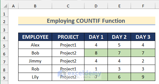
Method 3 – Using the COUNTIF Function in Conditional Formatting for More Than Two Columns
STEPS:
- Go to New Formatting Rule.
- Choose Use a formula to determine which cells to format.
- Enter the following formula.
=COUNTIF($D5:$F5,">4")>2- Go to Format option and select the cell background color.
- Click OK.
This is the output.
Formula Breakdown
The COUNTIF function will count the number of cells. If it is greater than 4 in the range $D5:$F5, it will return TRUE for exact matches; otherwise FALSE. The Conditional Formatting will apply the formula to the whole dataset.
Read more: How to Apply Conditional Formatting to Multiple Rows
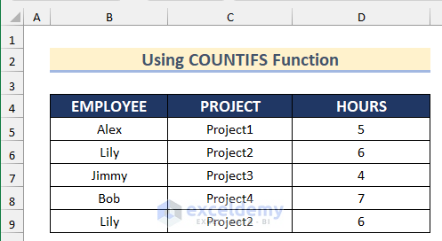
Method 4 – Find Duplicate Rows Based on Multiple Columns Using the COUNTIFS Function
The COUNTIFS function will count the number of cells from a range based on multiple criteria.
STEPS:
- Select the dataset.
- Go to the Home tab > Conditional Formatting > New Rule.
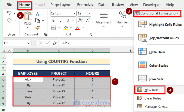
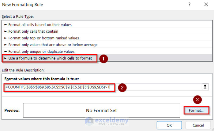
- In New Formatting Rule, select Use a formula to determine which cells to format.
- Enter the following formula.
=COUNTIFS($B$5:$B$9,$B5,$C$5:$C$9,$C5,$D$5:$D$9,$D5)>1- Go to Format.
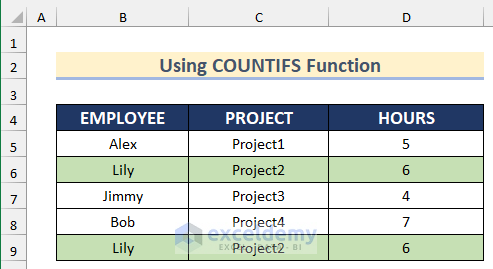
- Select the cell background color.
- Click OK.
This is the output.
Read more: Conditional Formatting Entire Column Based on Another Column
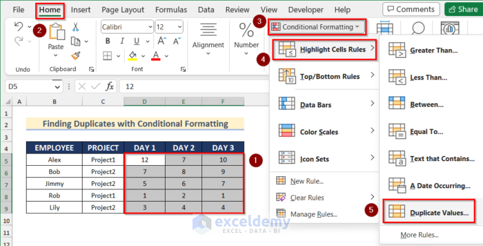
Method 5 – Using Conditional Formatting to Find Duplicates from Multiple Columns in Excel
STEPS:
- Select the range D5:F9.
- Go to the Home tab > Conditional Formatting.
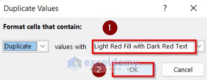
- Select Highlight Cells Rules >> click Duplicate Values.
- In Duplicate Values, select a color to indicate duplicate values.
- Click OK.
All duplicate values will be displayed.
Method 6 – Combining the OR, ISNUMBER, and SEARCH Functions in Conditional Formatting

STEPS:
- Select the dataset.
- Go to the Home tab > Conditional Formatting > New Rule.

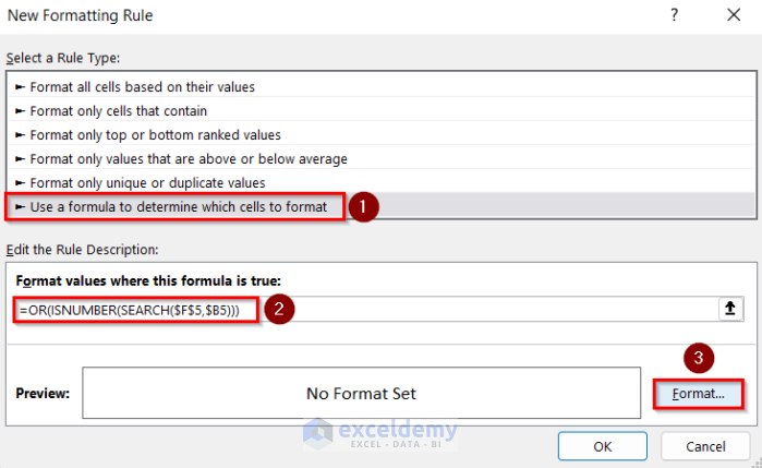
- In New Formatting Rule, choose Use a formula to determine which cells to format.
- Enter this formula.
=OR(ISNUMBER(SEARCH($F$5,$B5)))- Go to Format and select the cell background color.
- Click OK.
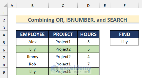
The duplicate rows are highlighted.
Formula Breakdown
- SEARCH($F$5,$B5): The SEARCH function will return the position of $F$5 in the lookup Range starting with $B5.
- ISNUMBER(SEARCH($F$5,$B5)): The ISNUMBER function will return the values as TRUE or FALSE.
- OR(ISNUMBER(SEARCH($F$5,$B5))): The OR function will alternate any of the text in the find_value Range.
Method 7 – Utilizing the SUM and COUNTIF Functions on Multiple Columns with Conditional Formatting
STEPS:
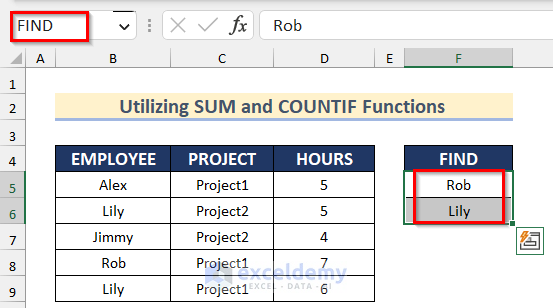
- Give the range F5:F6 a name. Here, ‘FIND’.
- Select the dataset.
- Go to the Home tab > Conditional Formatting > New Rule.
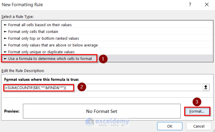
- In New Formatting Rule, choose Use a formula to determine which cells to format.
- Enter this formula.
=SUM(COUNTIF($B5,"*"&FIND&"*"))- Select Format.
- Choose the cell background color.
- Click OK.
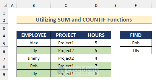
This is the output.
Formula Breakdown
- COUNTIF($B5,”*”&FIND&”*”): will count the number of cells that match only one criterion from the Range starting in $B5.
- SUM(COUNTIF($B5,”*”&FIND&”*”)): will match all criteria with the Range.
Method 8 – Using the AVERAGE Function in Conditional Formatting for Multiple Columns
STEPS:
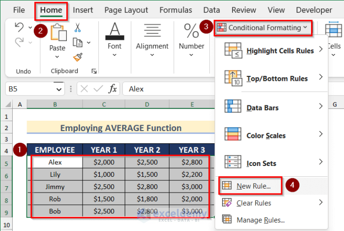
- Select the dataset.
- Go to the Home tab > Conditional Formatting > New Rule.
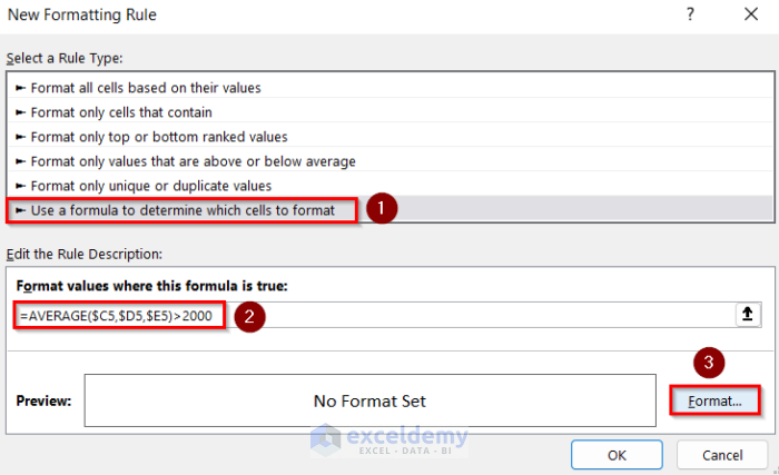
- In New Formatting Rule, choose Use a formula to determine which cells to format.
- Enter this formula.
=AVERAGE($C5,$D5,$E5)>2000- Go to Format and select the cell background color.
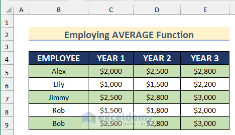
- Click OK.
This is the output.
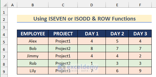
Method 9 – Changing Alternate Cell Color Using the ISEVEN or ISODD & ROW Functions with Conditional Formatting
STEPS:
- Select the dataset.
- Go to the Home tab >> click Conditional Formatting >> select New Rule.
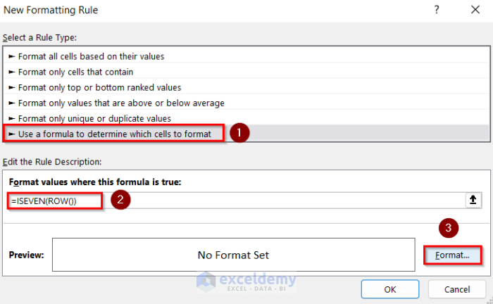
- In New Formatting Rule, choose Use a formula to determine which cells to format.
- Enter this formula.
=ISEVEN(ROW())- Go to Format and select the cell background color.
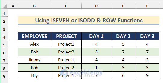
- Click OK.
All even rows are highlighted.
- To highlight he odd rows, enter this formula:
=ISODD(ROW())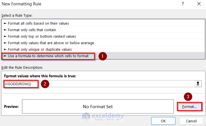
This is the output.
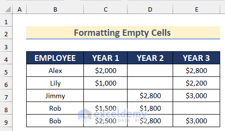
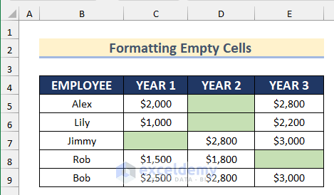
Method 10 – Formatting Empty Cells on Multiple Columns with Conditional Formatting in Excel
This dataset contains empty cells.
STEPS:
- Select the dataset.
- Go to the Home tab > Conditional Formatting > New Rule.
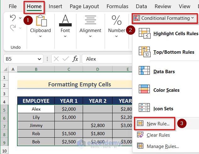
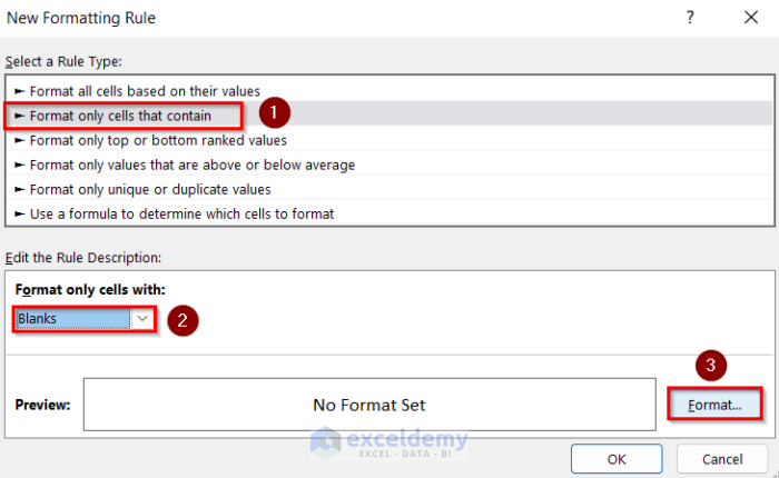
- In New Formatting Rule, choose ‘Format only cells that contain’.
- In ‘Format only cells with’, select Blanks.
- Go to Format option and select the cell background color.
- Click OK.
This is the result.
Practice Section
Practice on your own.

Download Practice Workbook
Download the workbook and exercise.
Related Readings
- How to Apply Different Types of Conditional Formatting in Excel
- How to Find External Links in Conditional Formatting in Excel
- How to Apply Conditional Formatting for Blank Cells in Excel
- How to Compare Two Columns Using Conditional Formatting in Excel
- How to Remove Conditional Formatting in Excel
- How to Remove Conditional Formatting but Keep the Format in Excel
- How to Do Conditional Formatting in Excel
- Conditional Formatting with Formula in Excel
<< Go Back to Conditional Formatting | Learn Excel
Get FREE Advanced Excel Exercises with Solutions!

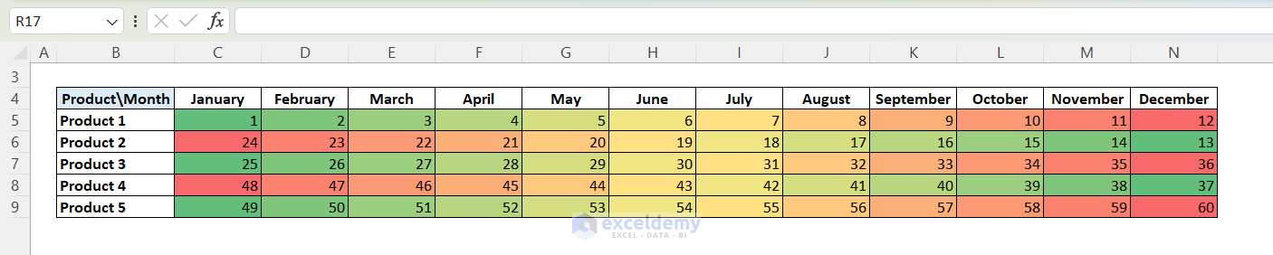
how about if i have months listed in a table, columns A – L ,and item numbers in the rows with sales for each month.
i want to make a conditional formatting rule for color scales, so it evaluates the ranking for each item across all columns so i can rank sales for each item by month. i could only get excel to evaluate by rows (so all item numbers were being ranked by each month instead of individula items being ranked by month).
if i selected a range and applied the rule, it ranked each column, not each row.
i had to write vba code to apply it row by row.
Dear Gary,
Thank you for sharing your problem with us. Yes, you are right that when you apply the conditional formatting (color scale) to the entire range,it ranks by each column, not by each row. Hence, in this case, to rank them by rows, you need to apply the conditional formatting to all the rows one by one. I have created a dataset based on your information and applied the conditional formatting to all the rows separately and got the expected result.
If you need to do this kind of stuff frequently, using VBA is indeed the best option as you mentioned.
Regards
Aniruddah
Team Exceldemy