How to Apply Alignment in Excel Conditional Formatting

We are familiar with diverse types of conditional formatting based on the criteria of various Excel users. However, in this article, we will discuss changing alignment using conditional formatting. Follow the steps and apply the necessary commands to apply alignment using Excel conditional formatting.

Apply Alignment with Conditional Formatting in Excel: 2 Examples

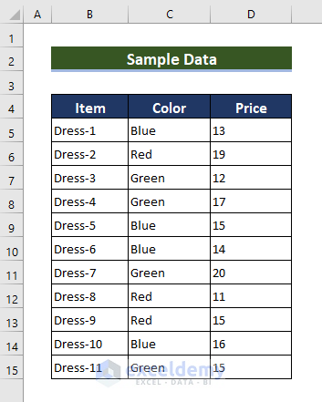
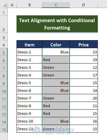
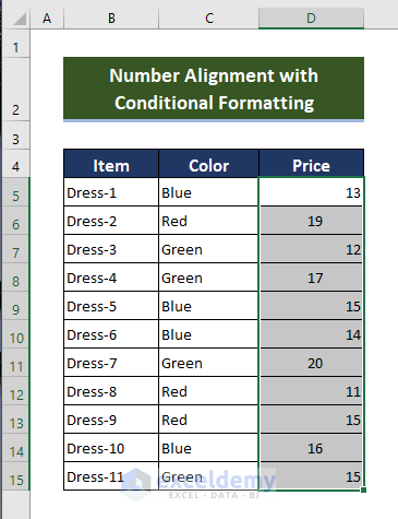
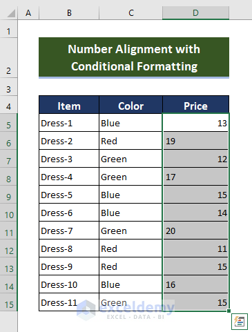
To demonstrate alignment using conditional formatting, we have a sample data table like the image below. In this data table, we have columns for Item, Color, and Price.

1. Apply Right and Left Alignment for Text That Meets a Criteria

In Excel, the default text alignment is left alignment. In this method, we will see that any cell that meets a certain criterion will change its alignment. This change in alignment will happen in the reverse order i.e.- if cells are on left they will align right.

Number Format for Right Aligned Text:

#,##0* ;;;* @

📌 Steps:

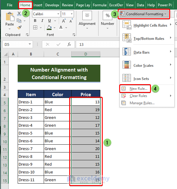
First of all, we will select the Color column and then go through the following procedures: Home >> Conditional Formatting >> New Rule.

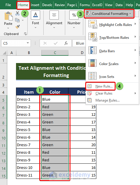
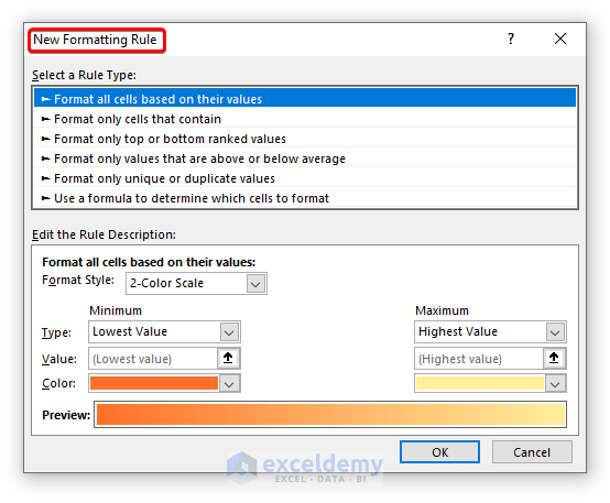
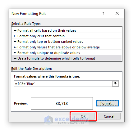
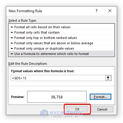
After clicking the New Rule, the New Formatting Rule pop-up will appear like the image below.

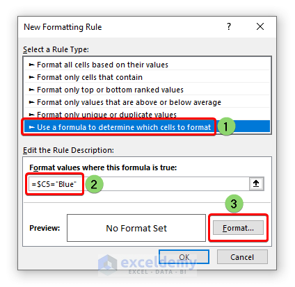
In the New Formatting Rule pop-up, we will select Use a formula to determine which cells to format >> enter the following formula in the box of Format values where this formula is true:

=$C5="Blue"

After that, we will select Format.

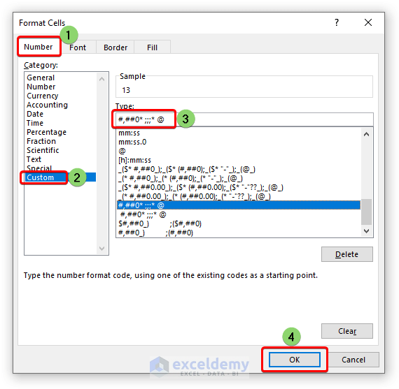
After selecting Format, Format Cells pop-up will appear.

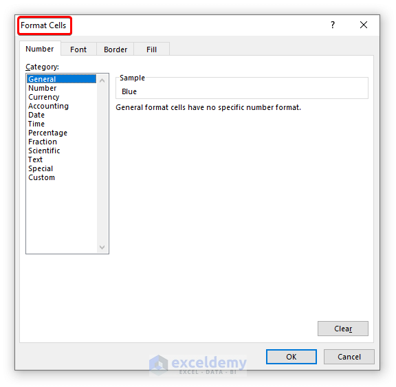
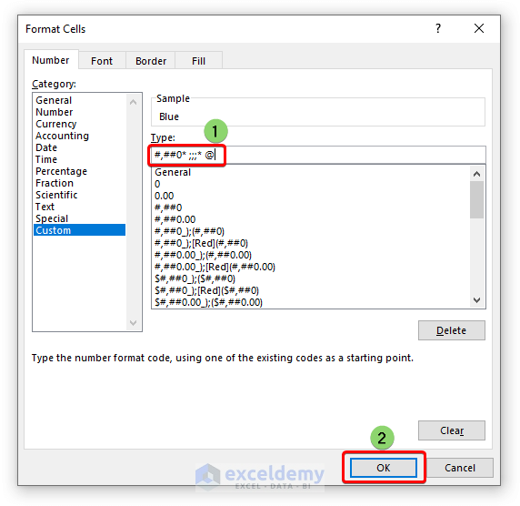
In the Format Cells pop-up, we will go to Custom under the Number tab. Then we will enter the following formula:

#,##0* ;;;* @

Now we will click OK.

Now again in the New Formatting Rule, we will hit the OK.

In the following image, we are observing that Blue has changed its alignment from left to right using conditional formatting.

2. Align Numbers to Right, Center, and Left with Excel Conditional Formatting

The default number alignment in Excel is the right alignment. In this procedure, each cell that fulfills a given set of criteria will have its alignment changed. This shift in alignment will occur in the opposite direction, so if cells are aligned to the right, they will align to the left.

For Center Alignment:

#,##0_) ;(#,##0)

For Left Alignment:

#,##0* ;;;* @

📌 Steps:

Now we will choose the Price column and proceed as follows: Home >> Conditional Formatting >> New Rule.

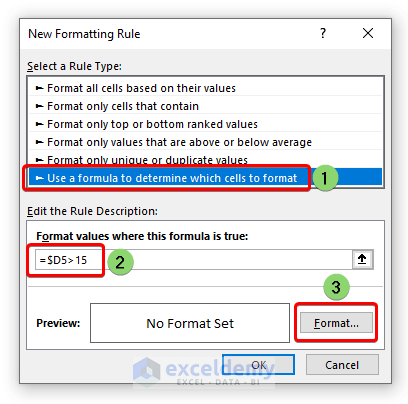
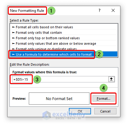
We will select Use a formula to determine which cells to format in New Formatting Rule >> enter the following formula in the box of Format values where this formula is true:

=$D5>15

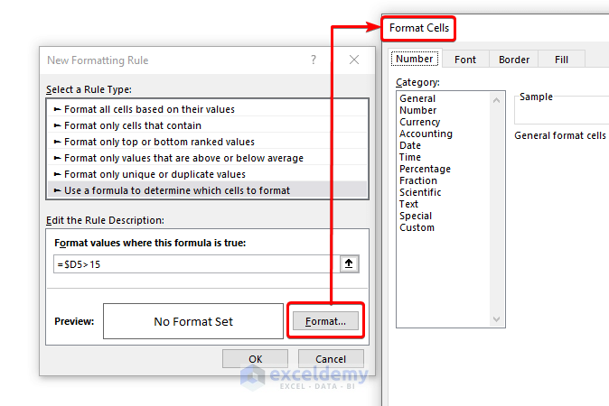
And then, we will press Format.

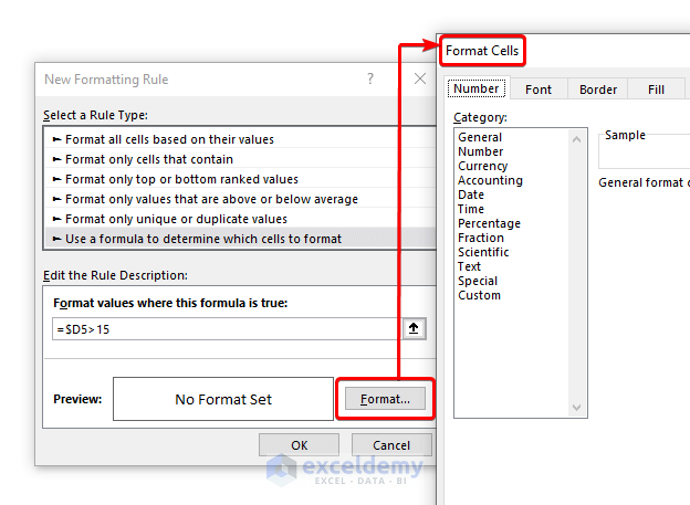
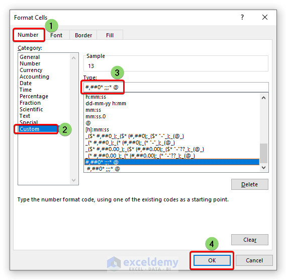
The Format Cells window will emerge once you pick Format like the following image.

We will select Custom from the Number menu in the Format Cells pop-up. Then we will plug in the following formula shown in the image below:

#,##0_) ;(#,##0)

And we will press OK.

Once again, we will select OK to complete the procedures.

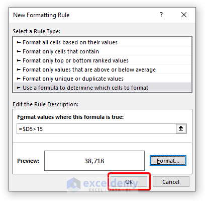
Now the result is in the following image that the cells containing values more than 15 have aligned in the middle.

Now, let us see how to align numbers to the left side. Do the following for that.

We will select Use a formula to determine which cells to format in the New Formatting Rule pop-up >> enter the following formula in the box of Format values where this formula is true:

=$D5>15

Following that, we will choose Format.

The Format Cells pop-up will appear once you select Format.

We will select Custom from the Number menu in the Format Cells pop-up. Then we will plug in the following formula:

#,##0* ;;;* @

We will now press the OK button.

For this time, we will now press the OK button in the New Formatting Rule.

Finally, in the accompanying figure, we can see that a number bigger than 15 has been shifted from right to left utilizing conditional formatting.

Note:

You can apply both rules and get the numbers in the left, middle, and right positions simultaneously.

Download Practice Workbook

You can download the practice workbook from the following download button.

Conditional Formatting Alignment.xlsx

Conclusion

Follow these steps and stages to excel in conditional formatting alignment. You are welcome to download the workbook and use it for your practice. If you have any questions, concerns, or suggestions, please leave them in the comments section.

<< Go Back to Conditional Formatting | Learn Excel

Get FREE Advanced Excel Exercises with Solutions!

Private Sub Worksheet_Change(ByVal Target As Range) Dim cell As Range Dim targetRange As Range Set targetRange = Me.Range("B2:B7") If Not Intersect(Target, targetRange) Is Nothing Then For Each cell In Intersect(Target, targetRange) If cell.Value = "Red" Then cell.HorizontalAlignment = xlLeft ElseIf cell.Value = "Blue" Then cell.HorizontalAlignment = xlCenter Else cell.HorizontalAlignment = xlRight End If Next cell End If End Sub

7 Comments

Richard Jan 18, 2024 at 8:48 PM

Curious how this is accomplished if you want your number values to have 2 or more decimal places
- Reply
  Abrar-ur-Rahman Niloy Jan 21, 2024 at 12:38 PM
  
  Hello Richard!
  
  You need to replace 0s in the format type with 0.00s.
  For example, instead of #,##0_) ;(#,##0) for center alignment, use #,##0.00_) ;(#,##0.00).
  
  Regards
  Niloy
  Team Exceldemy
M_curious Feb 9, 2024 at 4:40 AM

what is use to do a conditional alignment for a text?
Seems like the #,##0_) ;(#,##0) only works for number alignment
- Reply
  Lutfor Rahman Shimanto Jun 11, 2024 at 12:23 PM
  Hello there! Thanks for sharing an exciting problem. Since using the conditional formatting option for text alignment is impossible, you can only use an Excel VBA procedure.
  
  Note: The event procedure will trigger when range B2:B7 is changed. If the cell value is Red, it will apply left alignment. For Blue, it will be center alignment; for the other values, it will apply left alignment. You can modify the code based on your needs.
  
  Excel VBA Event Procedure:
```
Private Sub Worksheet_Change(ByVal Target As Range)

    Dim cell As Range

    Dim targetRange As Range
    Set targetRange = Me.Range("B2:B7")

    If Not Intersect(Target, targetRange) Is Nothing Then
        For Each cell In Intersect(Target, targetRange)

            If cell.Value = "Red" Then
                cell.HorizontalAlignment = xlLeft
            ElseIf cell.Value = "Blue" Then
                cell.HorizontalAlignment = xlCenter
            Else
                cell.HorizontalAlignment = xlRight
            End If
        Next cell
    End If

End Sub
```
  Hopefully, the solution will fulfil your goal. Download the attached solution workbook for a better understanding.
  
  DOWNLOAD SOLUTION WORKBOOK
  
  Regards
  Lutfor Rahman Shimanto
  Excel & VBA Developer
  ExcelDemy
- Reply
  Shamima Sultana Feb 12, 2024 at 1:27 PM
  
  Hello M-curious,
  
  To do a conditional formatting follow the steps of method 1. Instead of using custom option from format cells, you can use the Alignment options.
  Go to Format cells dialog box then from Alignment select any select any Alignments of your choice.
  
  Regards
  ExcelDemy
  - Reply
    ML Jun 11, 2024 at 4:40 AM
    
    Look at the screenshots in the article/post and alignment, when applying conditional formatting, isn’t an option – if it were we wouldn’t be looking for workarounds…
    - Lutfor Rahman Shimanto Jun 11, 2024 at 12:05 PM
      
      Dear, Thanks for pointing out the fact! You are right. The Alignment tab in the Format Cells dialog box is unavailable when setting up conditional formatting rules. So, using the conditional formatting option for text alignment is impossible.
      
      Don’t worry! There is an idea of using an Excel VBA event procedure. Please check the following:
      
      The event procedure will trigger when range B2:B7 is changed. If the cell value is Red, it will apply left alignment. For Blue, it will be center alignment; for the other values, it will apply left alignment.
      
      Excel VBA Event Procedure:
      
      Private Sub Worksheet_Change(ByVal Target As Range) Dim cell As Range Dim targetRange As Range Set targetRange = Me.Range("B2:B7") If Not Intersect(Target, targetRange) Is Nothing Then For Each cell In Intersect(Target, targetRange) If cell.Value = "Red" Then cell.HorizontalAlignment = xlLeft ElseIf cell.Value = "Blue" Then cell.HorizontalAlignment = xlCenter Else cell.HorizontalAlignment = xlRight End If Next cell End If End Sub
      
      Hopefully, the solution will fulfil your goal. I have attached the solution workbook as well. Good luck.
      
      DOWNLOAD SOLUTION WORKBOOK
      
      Regards
      Lutfor Rahman Shimanto
      Excel & VBA Developer
      ExcelDemy

How to Apply Alignment in Excel Conditional Formatting

Apply Alignment with Conditional Formatting in Excel: 2 Examples

1. Apply Right and Left Alignment for Text That Meets a Criteria

2. Align Numbers to Right, Center, and Left with Excel Conditional Formatting

Conclusion

Related Articles

Leave a reply Cancel reply