How to Remove Conditional Formatting but Keep the Format in Excel

If we remove conditional formatting from cells where it has been applied, Excel also removes the cell formats. In this article, we will demonstrate 2 different ways to remove conditional formatting but keep the cell formats.

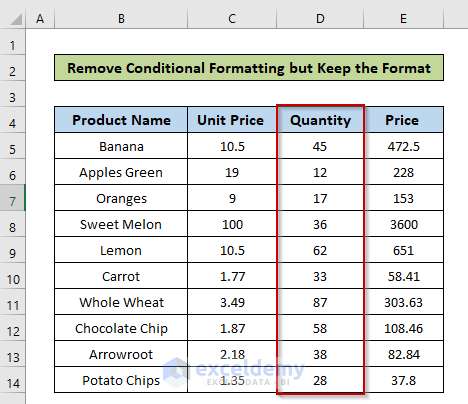
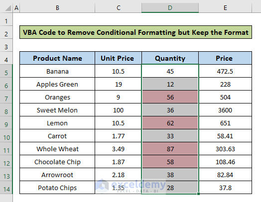
To illustrate our methods, we’ll use the dataset below, which contains a sale list including the product name, unit price, and sale quantity. We’ll first highlight the products that have a sale quantity of more than 50 using conditional formatting, then remove this formatting while preserving the general cell format.

To add the conditional formatting:

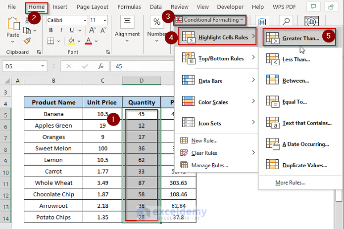
• Select the quantity column (cells D5:D14).
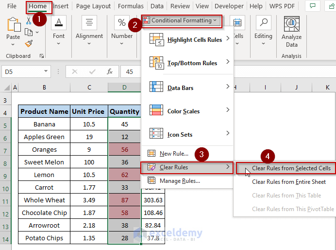
• From the Home tab on the ribbon, click Conditional Formatting.
• From the dropdown, choose Highlight Cells Rules.
• Then choose the Greater Than option.

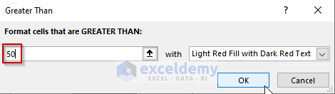
• In the Greater Than window, enter 50 and click OK.

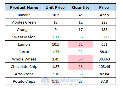
The cells having quantity greater than 50 now have a red background.

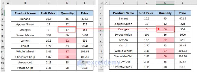
• To check the conditional formatting, change any cell value in the Quantity column that is less than 50 to a value greater than 50.

The following screenshot shows how the background color of cell D7 turns red when its value changed from 17 to 56.

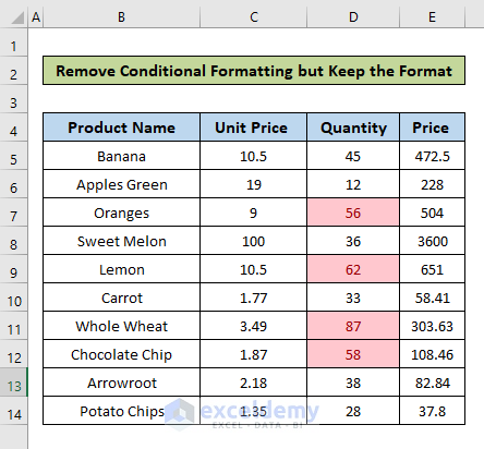
Remove Conditional Formatting and Keep the Format

Now we want to remove the conditional formatting rules while keeping the format at the same time. Using the standard procedure to remove conditional formatting rules, general formatting will also be removed.

Let’s remove the formatting rules but keep the formats.

Method 1 – Using the Office Clipboard

Steps:

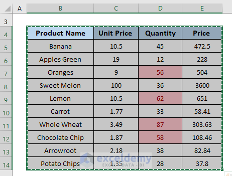
• Select the whole dataset.
• Press Ctrl + C to copy the selected cells.

• Select the cell to paste the copied cells.
• From the Home tab, click on the Clipboard icon.

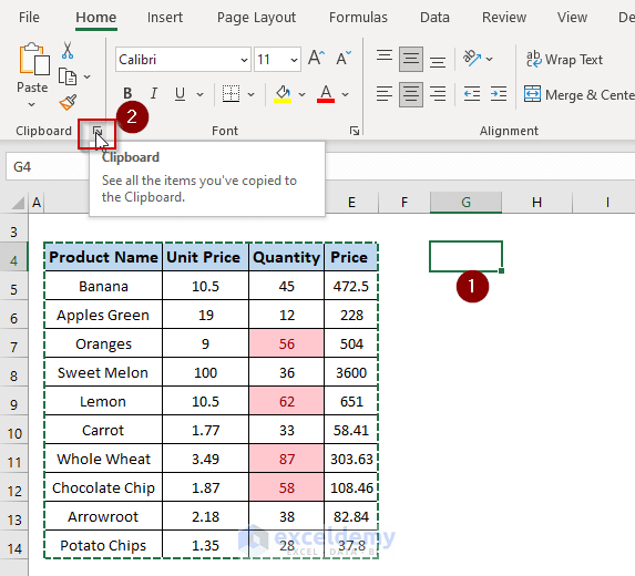
• Click on the copied item on the Clipboard panel.

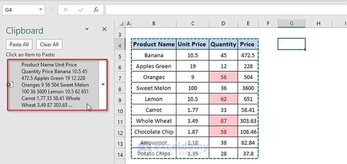
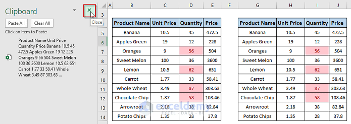
The copied cells are pasted at the specified location.

• Close the Clipboard panel.

• Delete the old dataset and reposition the new one.

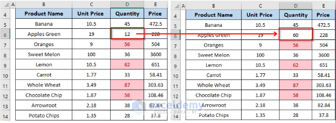
Now if we change the value of a cell in the Quantity column to greater than 50, the format doesn’t change.

Read More: How to Copy Conditional Formatting to Another Sheet

Method 2 – Running a VBA Code

Using VBA code, we can also remove conditional formatting while preserving the cell format.

Steps:

• Select the cells that are conditionally formatted (in our dataset, cells D5:D14).

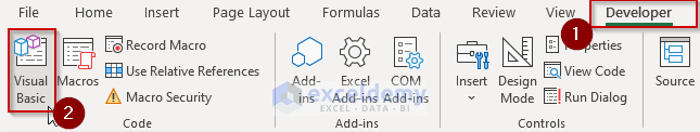
• Go to the Developer tab on the Excel Ribbon.
• Click the Visual Basic option.

• In the Visual Basic for Applications window, click the Insert dropdown to open a new Module.

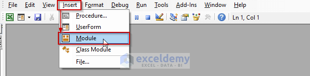
• Copy and the following code and paste it in the Module window:

Sub RemovConditionalFormattingButKeepFormat()
For Each cell In Selection
With cell
.Font.FontStyle = .DisplayFormat.Font.FontStyle
.Font.Strikethrough = .DisplayFormat.Font.Strikethrough
.Interior.Pattern = .DisplayFormat.Interior.Pattern
If .Interior.Pattern <> xlNone Then
.Interior.PatternColorIndex = .DisplayFormat.Interior.PatternColorIndex
.Interior.Color = .DisplayFormat.Interior.Color
End If
.Interior.TintAndShade = .DisplayFormat.Interior.TintAndShade
.Interior.PatternTintAndShade = .DisplayFormat.Interior.PatternTintAndShade
End With
Next
Selection.FormatConditions.Delete
End Sub

• Press F5 to run the code.

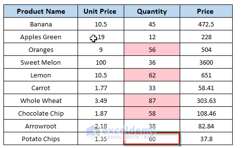
The conditional formatting is removed while keeping the formatting as it was. Now if we change the value of a cell in the Quantity column to greater than 50, its format won’t change.

Notes

• In the VBA code, we used the DisplayFormat property to keep the cell format as it is. We also applied the FormatConditons object to delete the conditional formatting.
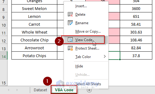
• To view the code, click the right button on the sheet name and select View Code.

Download Practice Workbook

Related Articles

• How to Apply Different Types of Conditional Formatting in Excel
• How to Find External Links in Conditional Formatting in Excel
• How to Apply Conditional Formatting for Blank Cells in Excel
• How to Apply Conditional Formatting on Multiple Columns in Excel
• How to Compare Two Columns Using Conditional Formatting in Excel
• How to Remove Conditional Formatting in Excel
  
• How to Do Conditional Formatting in Excel
• Conditional Formatting with Formula in Excel

<< Go Back to Conditional Formatting | Learn Excel