How to Use Formula with Excel Conditional Formatting
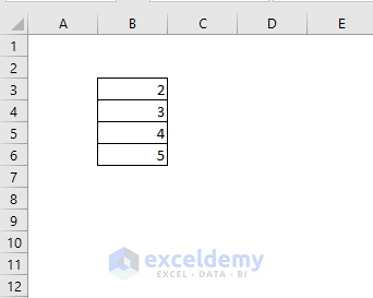
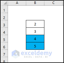
In the following image, we have a very simple dataset. With Excel conditional formatting with formula, we will highlight the values that are greater than 3.
Steps:
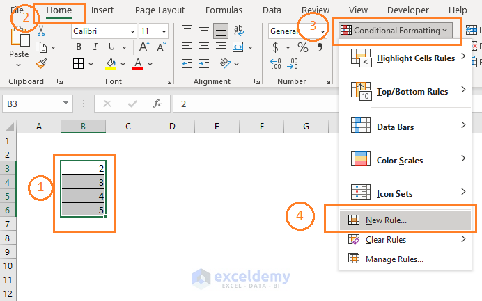
- Select the range of cells.
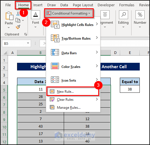
- Go to Home, click on the Conditional Formatting drop-down, then select New Rule from the drop-down menu.
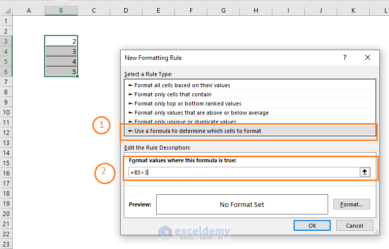
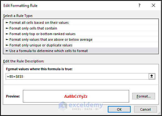
- The New Formatting Rule dialog box appears.
- Select Use a formula to determine which cells to format
- In the Format values where this formula is true: field, we input this formula: =B3>3
- Click on the Format command. Choose a Fill Color and click OK.
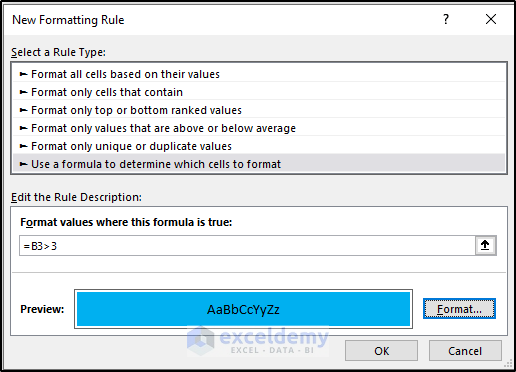
- Click OK in the dialog box.
The range on the spreadsheet was B3:B6. It will now look like this.
Using Conditional Formatting with Formula in Excel: 21 Examples
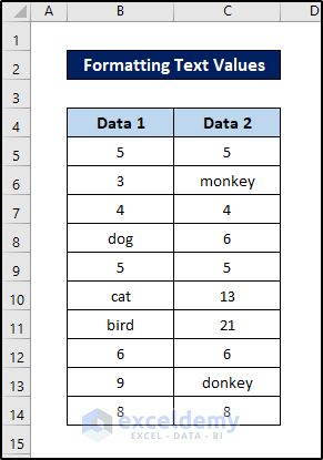
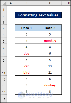
Example 1 – Format Text Values
Let’s consider this dataset containing both numeric and string values in it.
Steps:
- Select all the cells in the dataset excluding headers.
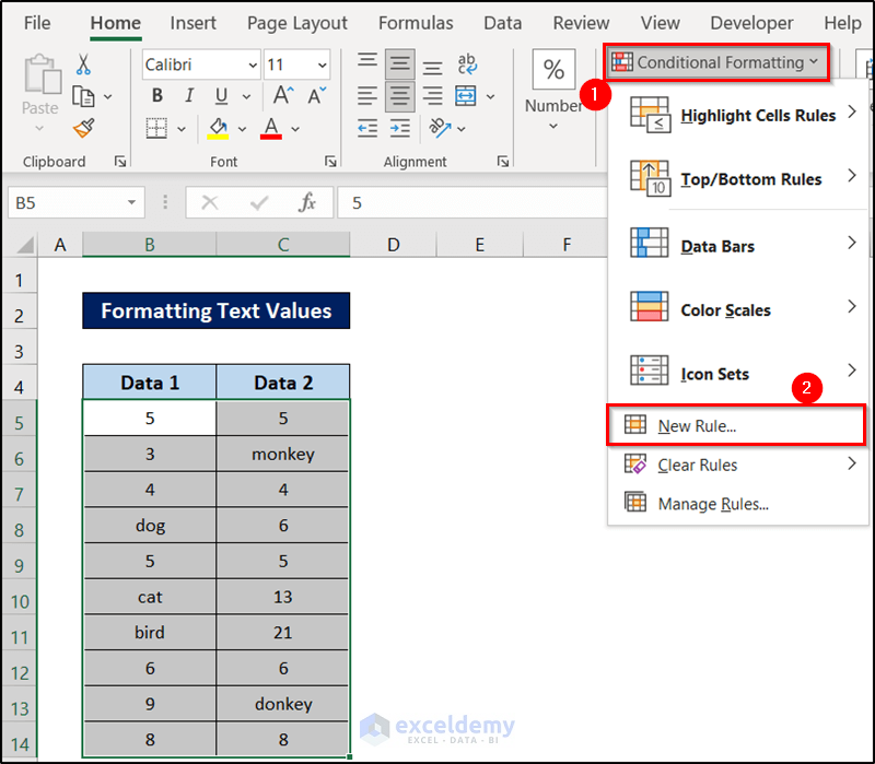
- Go to the Home tab on your ribbon.
- Select Conditional Formatting from the Styles group section.
- Select New Rule from the drop-down menu.
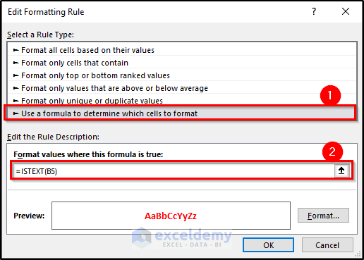
- In the Formatting Rule box, select the Use a formula to determine which cells to format option under Select a Rule Type.
- Insert the following formula in Format values where this formula is true.
=ISTEXT(B5)
- Select your preferred format type.
- Click on OK.
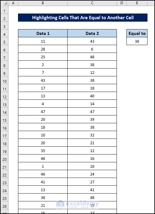
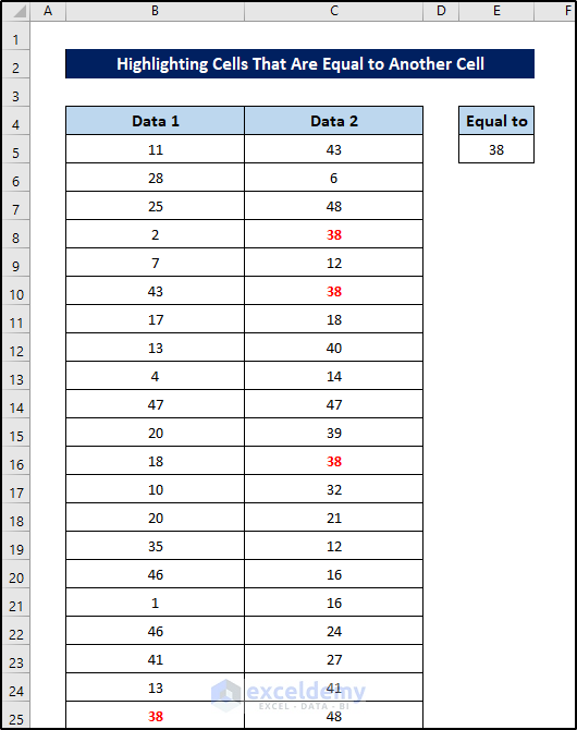
Example 2 – Highlight Cells That Are Equal to Another Cell
We are going to format the values that match the cell value of E5.
Steps:
- Select all the cells in the dataset excluding headers.
- Go to the Home tab on your ribbon.
- Select Conditional Formatting from the Styles group section.
- Select New Rule from the drop-down menu.
- In the Formatting Rule box, select the Use a formula to determine which cells to format option under Select a Rule Type.
- Insert the following formula in the Format values where this formula is true.
=B5=$E$5
- Select your preferred format type.
- Click on OK.
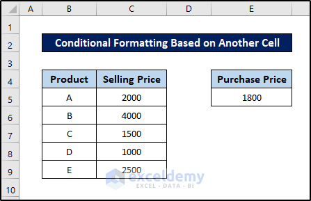
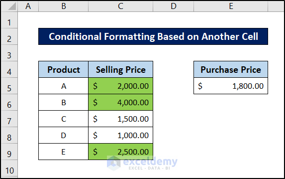
Example 3 – Conditional Formatting in Excel Based on Another Cell
We will format a dataset based on whether it is larger or smaller than another cell’s value.
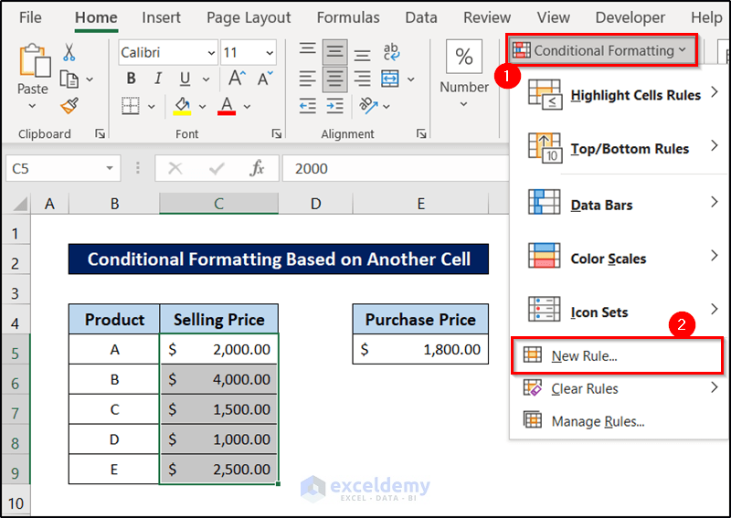
Steps:
- Select all the cells in the dataset excluding headers.
- Go to the Home tab on your ribbon.
- Select Conditional Formatting from the Styles group section.
- Select New Rule from the drop-down menu.
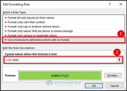
- In the Formatting Rule box, select the Use a formula to determine which cells to format option under Select a Rule Type.
- Insert the following formula in the Format values where this formula is true.
=C5>$E$5
- Select your preferred format type.
- Click on OK.
- You can repeat the same process for the lower values and end up with a dataset like this.
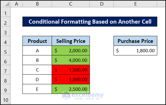
Read More: How to Do Conditional Formatting Based on Another Cell in Excel
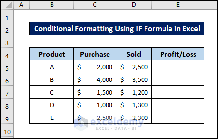
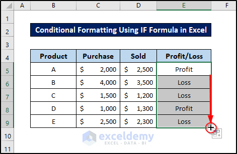
Example 4 – Conditional Formatting Using the IF Formula in Excel
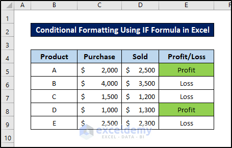
We’ll determine whether the product turned a profit and highlight the cell.
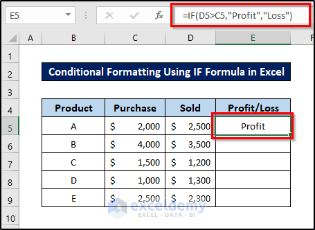
Steps:
- Select cell E5 and insert the following formula.
=IF(D5>C5,"Profit","Loss")
- Hit Enter.
- Click and drag the fill handle icon to the end of the column to replicate the formula for the rest of the cells.
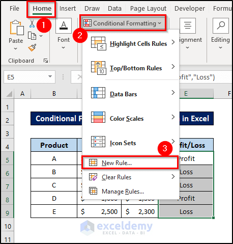
- Select all the cells in the dataset excluding headers.
- Go to the Home tab on your ribbon.
- Select Conditional Formatting from the Styles group section.
- Select New Rule from the drop-down menu.
- In the Formatting Rule box, select the Use a formula to determine which cells to format option under Select a Rule Type.
- Insert the following formula in the Format values where this formula is true.
=E5="Profit"
- Select your preferred format type.
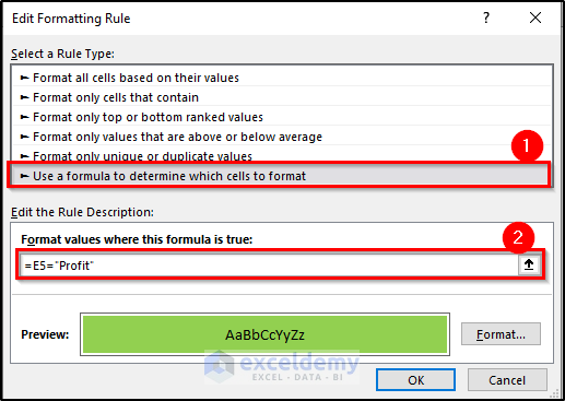
- Click on OK.
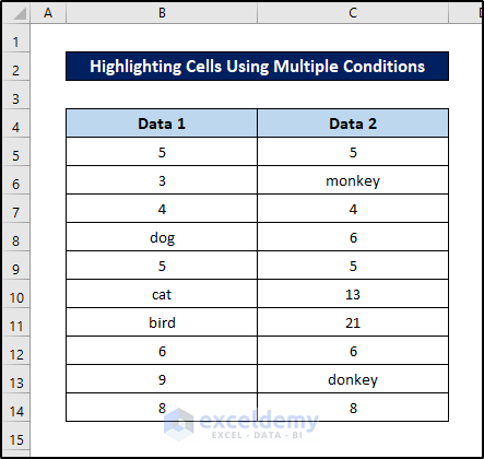
Example 5 – Highlight Cells Using Multiple Conditions
Let’s go back to the first dataset. We are going to highlight all the cells that are either 5, 6, or contain the text “cat”.
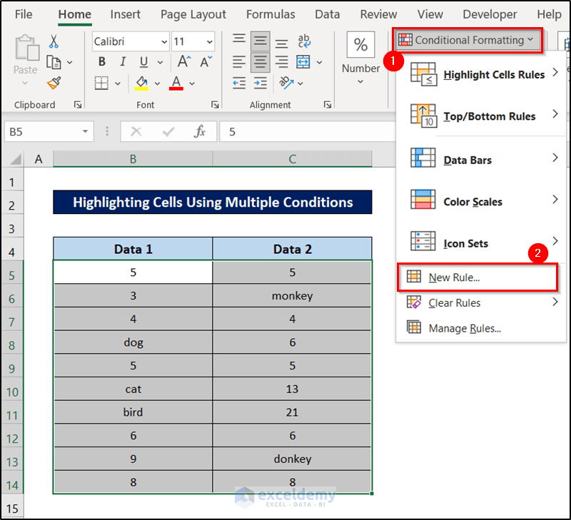
Steps:
- Select all the cells in the dataset excluding headers.
- Go to the Home tab on your ribbon.
- Select Conditional Formatting from the Styles group section.
- Select New Rule from the drop-down menu.
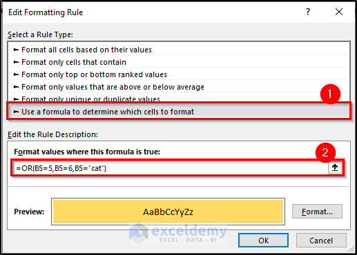
- In the Edit Formatting Rule box, select the Use a formula to determine which cells to format option under Select a Rule Type.
- Insert the following formula in the Format values where this formula is true.
=OR(B5=5,B5=6,B5="cat")
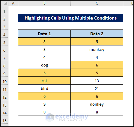
- Select your preferred format type.
- Click on OK.
Read More: Applying Conditional Formatting for Multiple Conditions in Excel
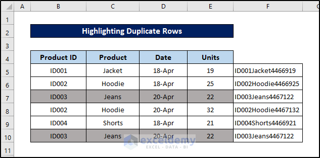
Example 6 – Highlight Duplicate Rows
We are going to highlight cells in the whole rows where the whole row matches with another one.
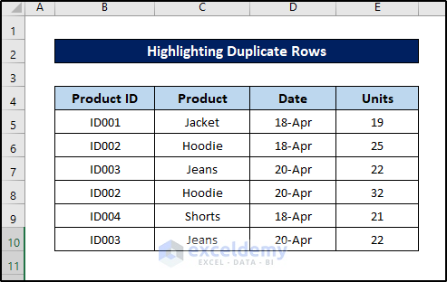
We can see the third and sixth row fully match.
Steps:
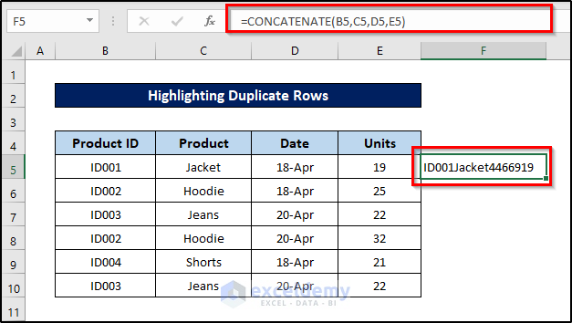
- Select cell F5 and use the following formula.
=CONCATENATE(B5,C5,D5,E5)
- Press Enter.
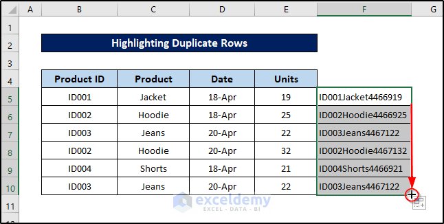
- Select the cell again and click and drag the fill handle icon down to fill up the rest of the cells with the formula for their references.
- Select the range B5:B10.
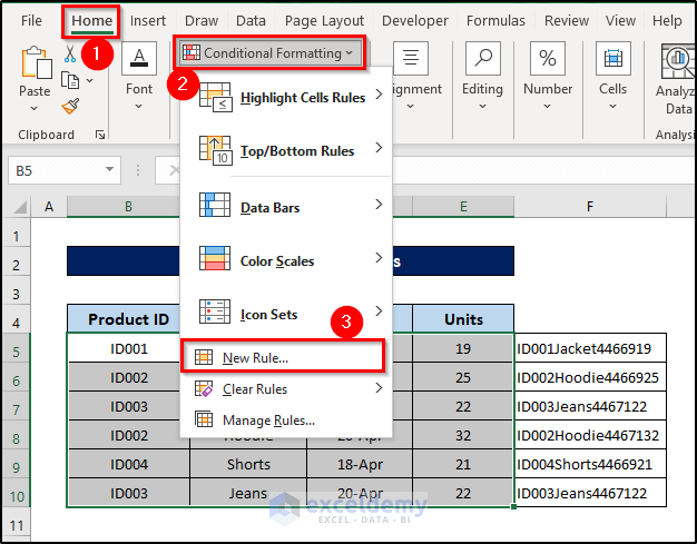
- Go to the Home tab on your ribbon.
- Select Conditional Formatting from the Styles group section.
- Select New Rule from the drop-down menu.
- In the Edit Formatting Rule box, select the Use a formula to determine which cells to format option under Select a Rule Type.
- Insert the following formula in the Format values where this formula is true.
=COUNTIF($F$5:$F$10,$F5)>1
- Select your preferred format type.
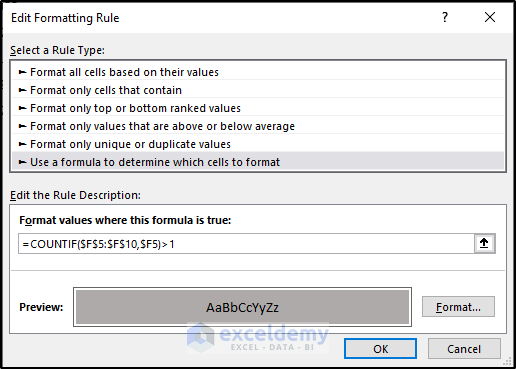
- Click on OK.
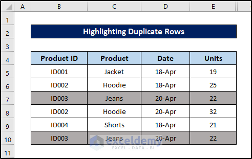
- Right-click on the column header of F and select Hide from the context menu.
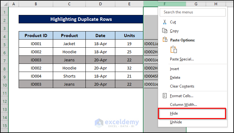
Here’s the sheet.
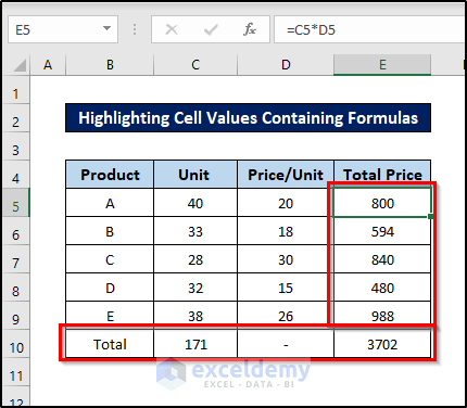
Example 7 – Highlight Cells Containing Formulas
Let’s take a look at a dataset that contains formulas to complete.
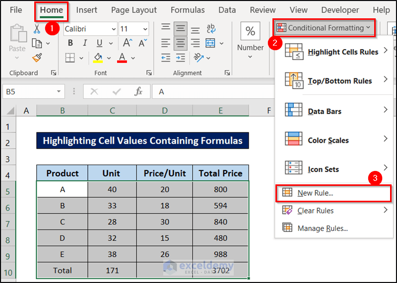
Steps:
- Select all the cells in the dataset excluding headers.
- Go to the Home tab on your ribbon.
- Select Conditional Formatting from the Styles group section.
- Select New Rule from the drop-down menu.
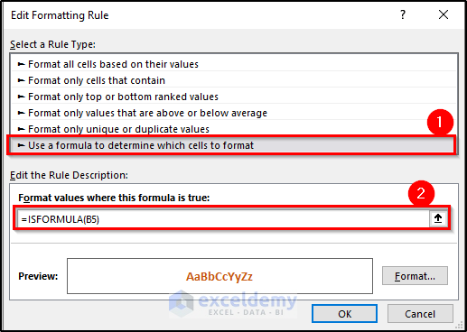
- In the Formatting Rule box, select the Use a formula to determine which cells to format option under Select a Rule Type.
- Insert the following formula in the Format values where this formula is true.
=ISFORMULA(B5)
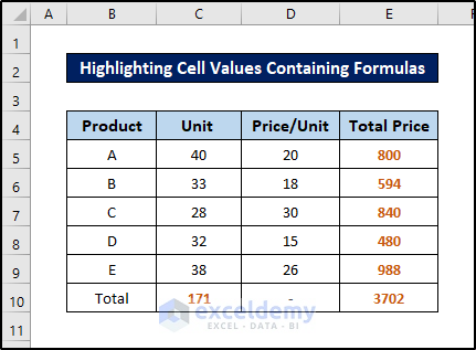
- Select your preferred format type.
- Click on OK.
Read More: How to Format Cell Based on Formula in Excel
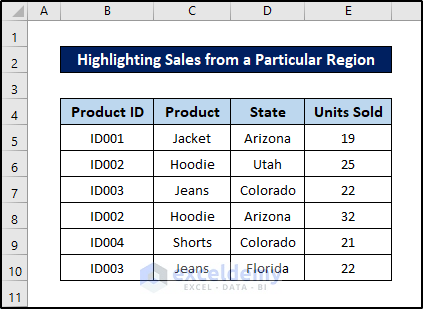
Example 8 – Highlight Sales from a Particular Region
We are going to highlight sales from a dataset that belongs to a particular region.
Steps:
- Select all the cells in the dataset excluding headers.
- Go to the Home tab on your ribbon.
- Select Conditional Formatting from the Styles group section.
- Select New Rule from the drop-down menu.
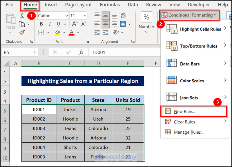
- In the Formatting Rule box, select the Use a formula to determine which cells to format option under Select a Rule Type.
- Insert the following formula in the Format values where this formula is true.
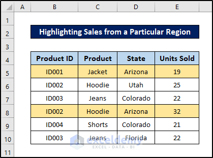
=$D5="Arizona"
- Select your preferred format type.
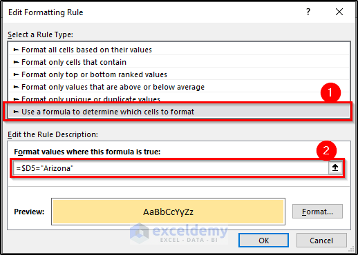
- Click on OK.
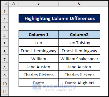
Example 9 – Highlight Column Differences
We can also highlight rows that have different columns than their adjacent ones.
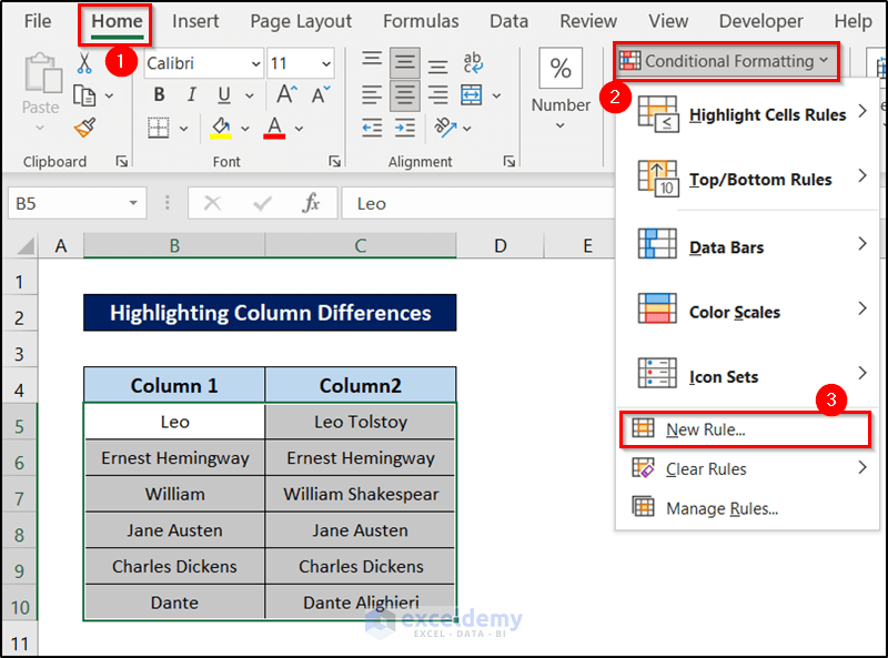
Steps:
- Select all the cells in the dataset excluding headers.
- Go to the Home tab on your ribbon.
- Select Conditional Formatting from the Styles group section.
- Select New Rule from the drop-down menu.
- In the Formatting Rule box, select the Use a formula to determine which cells to format option under Select a Rule Type.
- Insert the following formula in the Format values where this formula is true.
=$B5<>$C5
- Select your preferred format type.
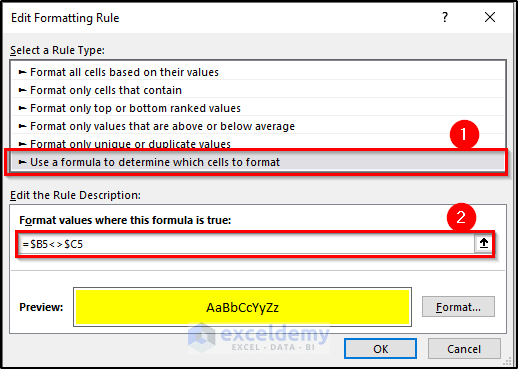
- Click on OK.
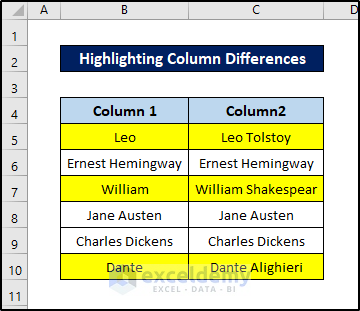
Read More: How to Compare Two Columns Using Conditional Formatting in Excel
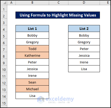
Example 10 – Using a Formula to Highlight Missing Values
We will use a formula to highlight missing values in conditional formatting in Excel.
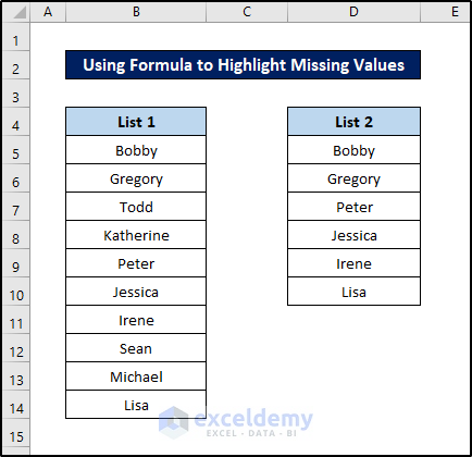
Steps:
- Select all the cells in the dataset excluding headers.
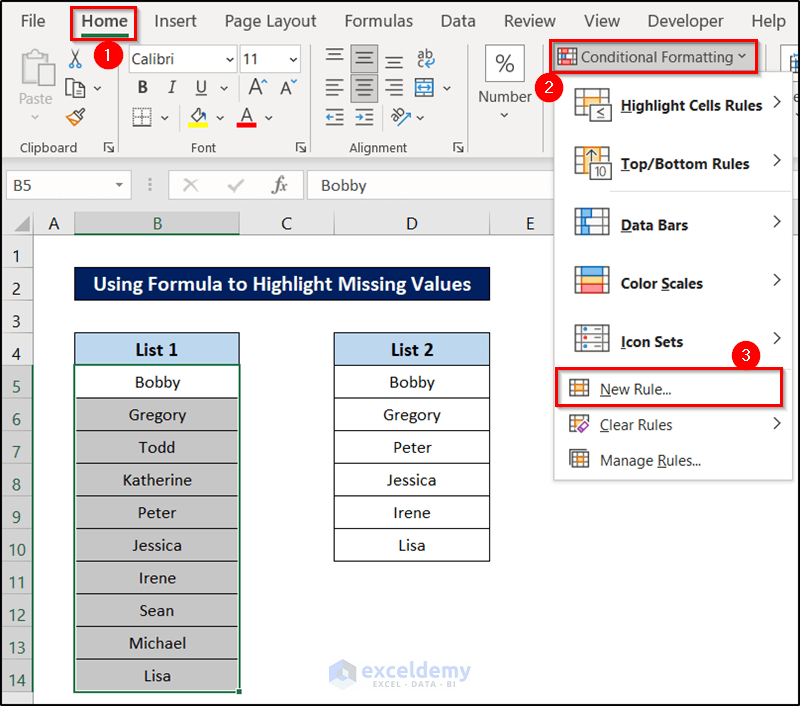
- Go to the Home tab on your ribbon.
- Select Conditional Formatting from the Styles group section.
- Select New Rule from the drop-down menu.
- In the Formatting Rule box, select the Use a formula to determine which cells to format option under Select a Rule Type.
- Insert the following formula in the Format values where this formula is true.
=COUNTIF($D$5:$D$10,$B5)=0
- Select your preferred format type.
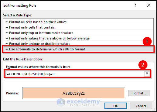
- Click on OK.
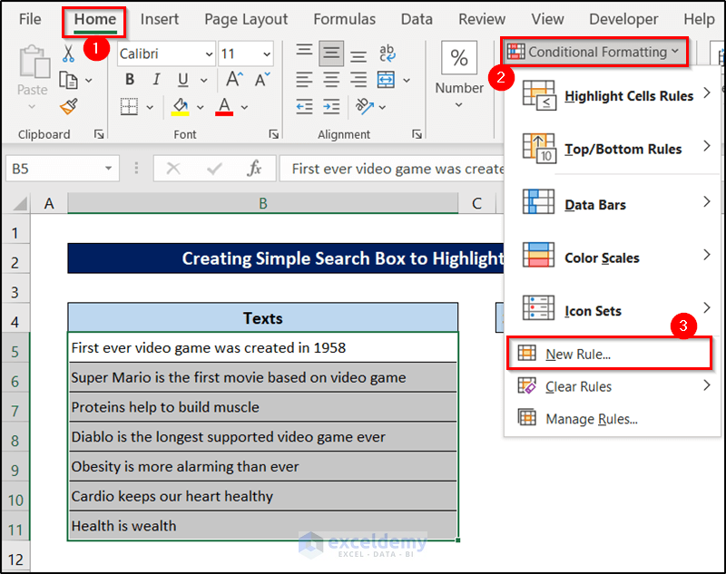
Example 11 – Creating a Simple Search Box to Highlight Cells
We will put a value in cell E4, and Excel will highlight the value in the range, all with the conditional formatting with the formula method.

Steps:
- Select all the cells in the dataset excluding headers.
- Go to the Home tab on your ribbon.
- Select Conditional Formatting from the Styles group section.
- Select New Rule from the drop-down menu.
- In the Formatting Rule box, select the Use a formula to determine which cells to format option under Select a Rule Type.
- Insert the following formula in the Format values where this formula is true.
=ISNUMBER(SEARCH($E$4,B5))
- Select your preferred format type.
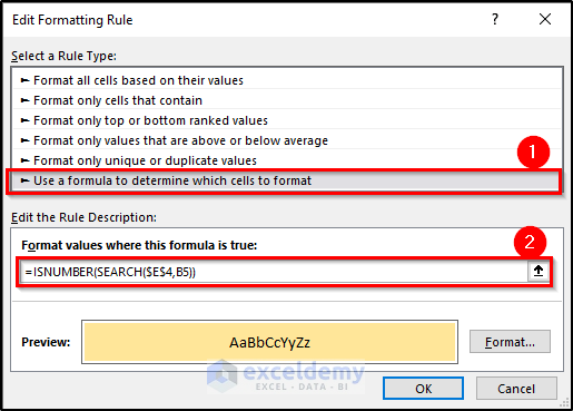
- Click on OK.
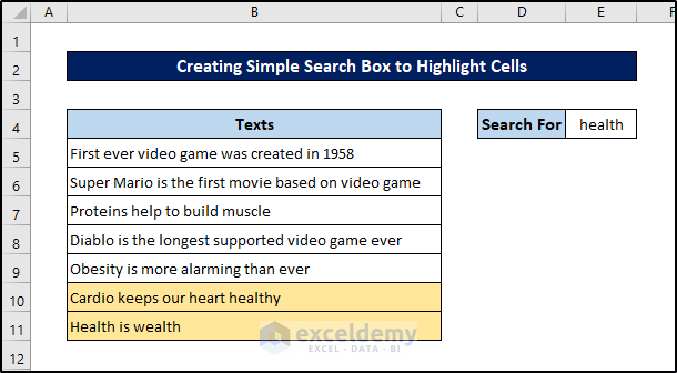
The texts containing the word game will be marked.

If we change the value in cell E4, the highlights will change.
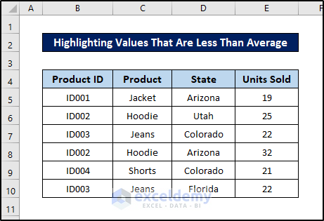
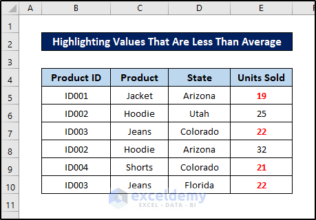
Example 12 – Highlight Values That Are Lower Than Average
Let’s revisit one of the datasets from before.
Steps:
- Select all the cells in the dataset excluding headers.
- Go to the Home tab on your ribbon.
- Select Conditional Formatting from the Styles group section.
- Select New Rule from the drop-down menu.

- In the Formatting Rule box, select the Use a formula to determine which cells to format option under Select a Rule Type.
- Insert the following formula in the Format values where this formula is true.
=E5<AVERAGE($E$5:$E$10)
- Select your preferred format type.
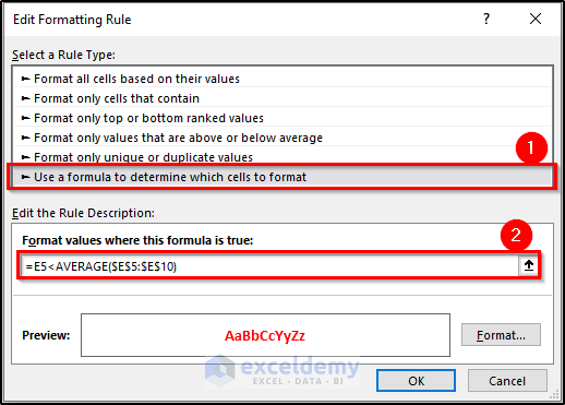
- Click on OK.
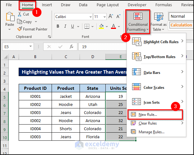
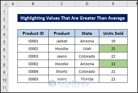
Example 13 – Highlight Values That Are Greater Than Average
Steps:
- Select all the cells in the dataset excluding headers.
- Go to the Home tab on your ribbon.
- Select Conditional Formatting from the Styles group section.
- Select New Rule from the drop-down menu.
- In the Edit Formatting Rule box, select the Use a formula to determine which cells to format option under Select a Rule Type.
- Insert the following formula in the Format values where this formula is true.
=E5>AVERAGE($E$5:$E$10)
- Select your preferred format type.
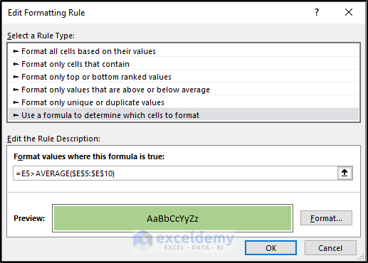
- Click on OK.
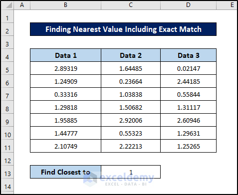
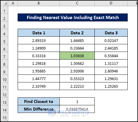
Example 14 – Find the Nearest Value Including the Exact Match
We are going to find the value that is closest to the one in cell C13. If there is the same value in the dataset, it will highlight that cell instead of the closest value.
Steps:
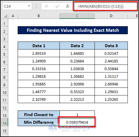
- We need to find the smallest difference from this value in that set of data. For that, select cell C14 and insert the following formula.
=MIN(ABS(B5:D11-(C13)))
- Press Enter.
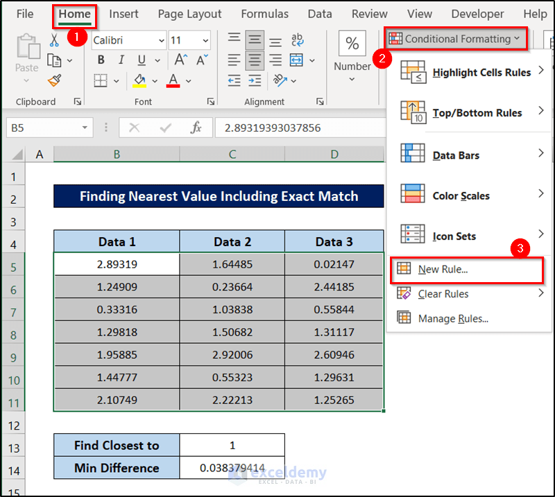
- Select all the cells in the dataset excluding headers.
- Go to the Home tab on your ribbon.
- Select Conditional Formatting from the Styles group section.
- Select New Rule from the drop-down menu.
- In the Formatting Rule box, select the Use a formula to determine which cells to format option under Select a Rule Type.
- Insert the following formula in the Format values where this formula is true.
=OR(B5=$C$13-$C$14,B5=$C$13+$C$14)
- Select your preferred format type.
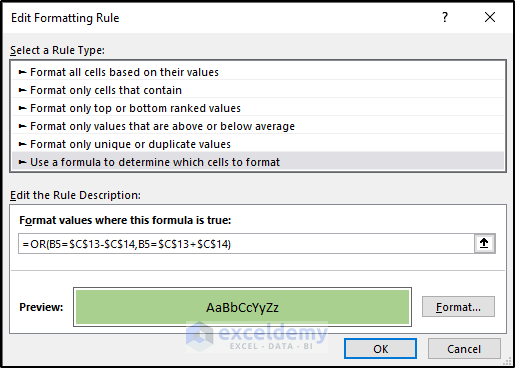
- Click on OK.
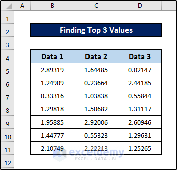
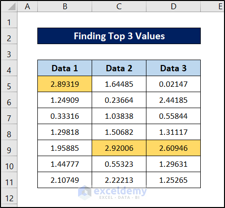
Example 15 – Find the Top 3 Values
Let’s go back to the random set of data.
Steps:
- Select all the cells in the dataset excluding headers.
- Go to the Home tab on your ribbon.
- Select Conditional Formatting from the Styles group section.
- Select New Rule from the drop-down menu.

- In the Formatting Rule box, select the Use a formula to determine which cells to format option under Select a Rule Type.
- Insert the following formula in the Format values where this formula is true.
=B5>=LARGE($B$5:$D$11,3)
- Select your preferred format type.
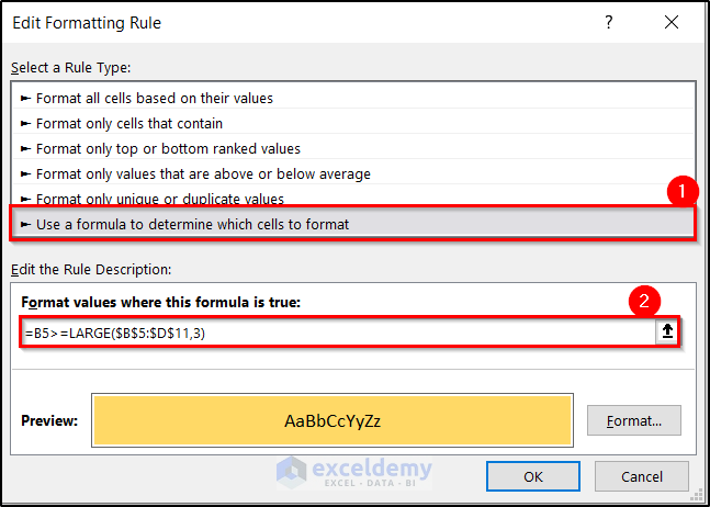
- Click on OK.
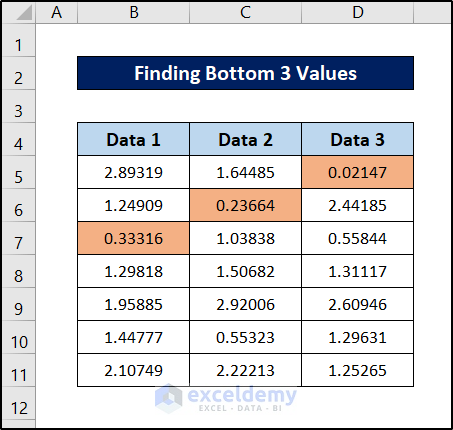
Example 16 – Find the Bottom 3 Values
Steps:
- Select all the cells in the dataset excluding headers.
- Go to the Home tab on your ribbon.
- Select Conditional Formatting from the Styles group section.
- Select New Rule from the drop-down menu.
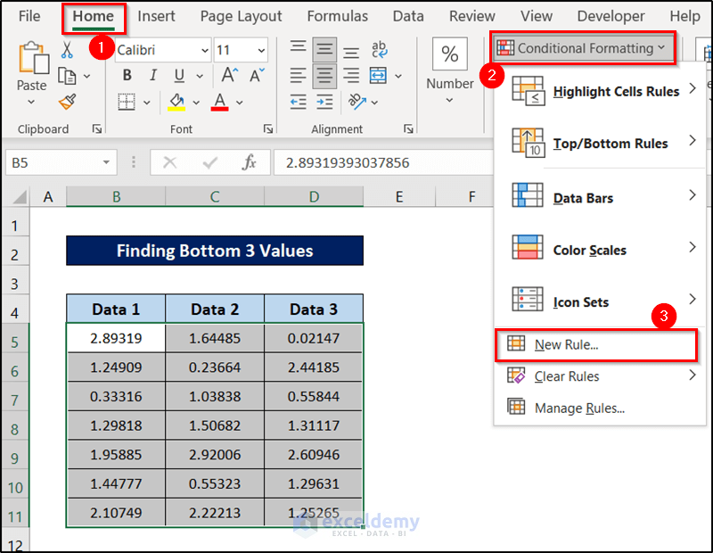
- In the Formatting Rule box, select the Use a formula to determine which cells to format option under Select a Rule Type.
- Insert the following formula in the Format values where this formula is true.
=B5<=SMALL($B$5:$D$11,3)
- Select your preferred format type.

- Click on OK.
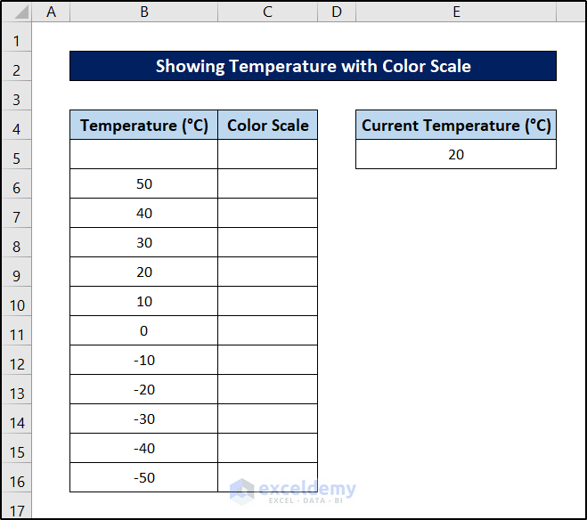
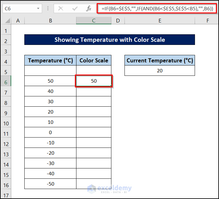
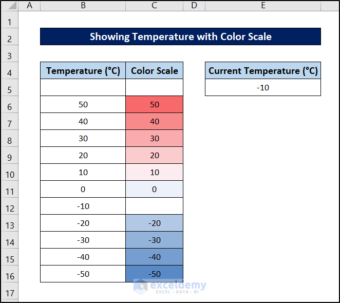
Example 17 – Show the Temperature with a Color Scale
We have two columns because we will use a formula to change the color based on the input in cell E5. There is a blank row at the start of the dataset. We will change the color scheme of temperature values based on the current temperature.
Steps:
- Select cell C6 and insert the following formula in it.
=IF(B6=$E$5,"",IF(AND(B6<$E$5,$E$5<B5),"",B6))
- Press Enter.
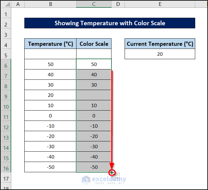
- Select the cell again and click and drag the fill handle icon to replicate the formula for the rest of the cells in the column.
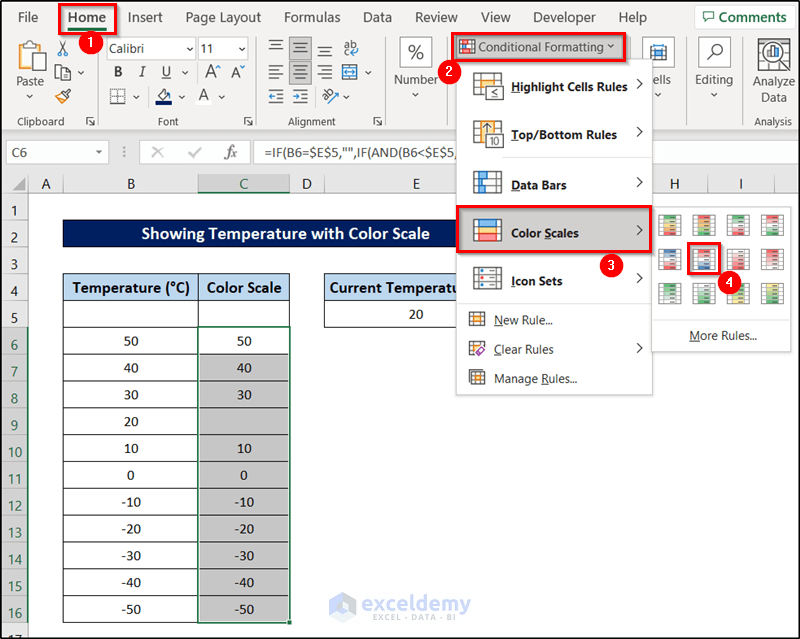
- Go to Conditional Formatting from the Styles group of the Home section.
- Hover over Color Scales.
- Select your preferred color scale.
- The temperature scale for conditional formatting based on the formula for current temperature will now be complete.
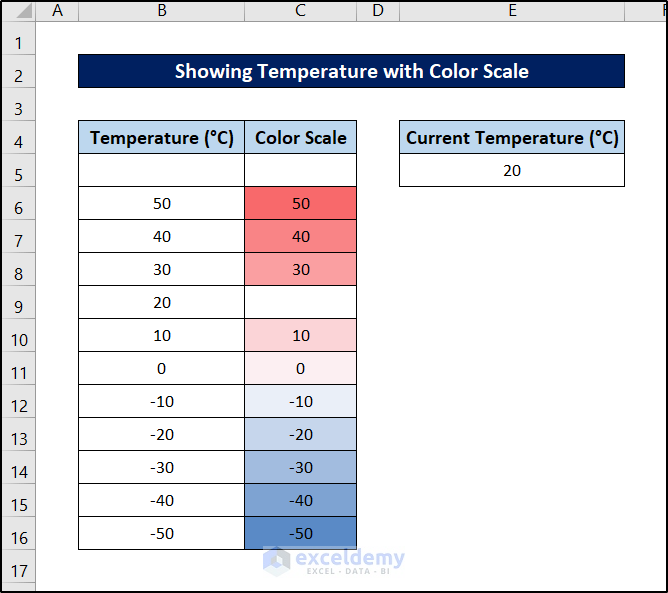
- If we change the value of the current temperature in cell E5, the temperature scale will change accordingly.
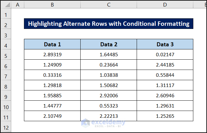
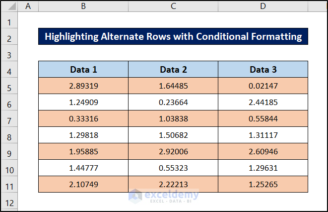
Example 18 – Highlight Alternate Rows with Conditional Formatting
We will highlight alternate rows with a color.
Steps:
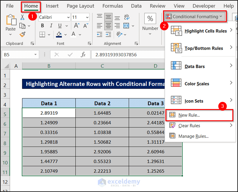
- Select all the cells in the dataset excluding headers.
- Go to the Home tab on your ribbon.
- Select Conditional Formatting from the Styles group section.
- Select New Rule from the drop-down menu.
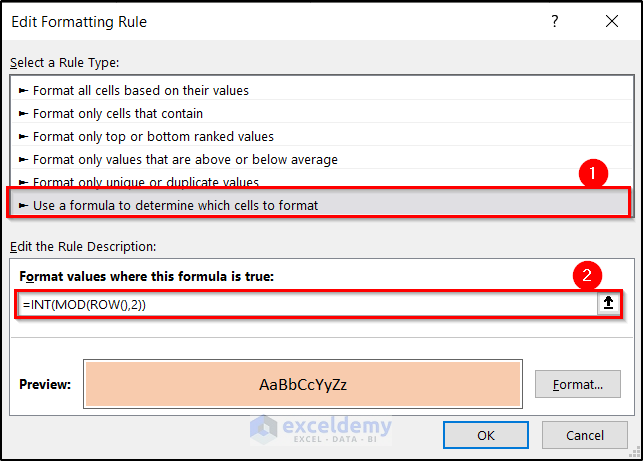
- In the Formatting Rule box, select the Use a formula to determine which cells to format option under Select a Rule Type.
- Insert the following formula in the Format values where this formula is true.
=INT(MOD(ROW(),2))
- Select your preferred format type.
- Click on OK.
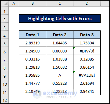
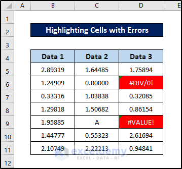
Example 19 – Highlight Cells with Error
Consider this simple dataset.
Steps:
- Select all the cells in the dataset excluding headers.
- Go to the Home tab on your ribbon.
- Select Conditional Formatting from the Styles group section.
- Select New Rule from the drop-down menu.
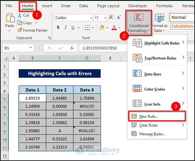
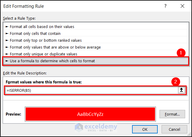
- In the Edit Formatting Rule box, select the Use a formula to determine which cells to format option under Select a Rule Type.
- Insert the following formula in the Format values where this formula is true.
=ISERROR(B5)
- Select your preferred format type.
- Click on OK.
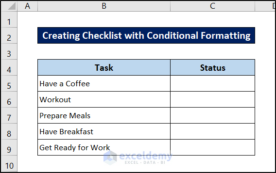
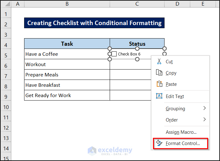
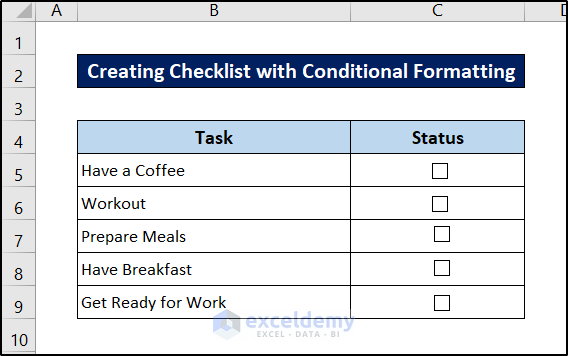
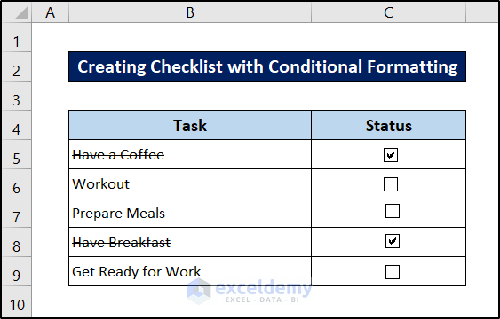
Example 20 – Create a Checklist with Conditional Formatting
We will make a checklist beside a set of data. With the options checked, the original data will change its format.
Steps:
- Go to the Developer tab on your ribbon.
- Select Insert from the Controls group section.
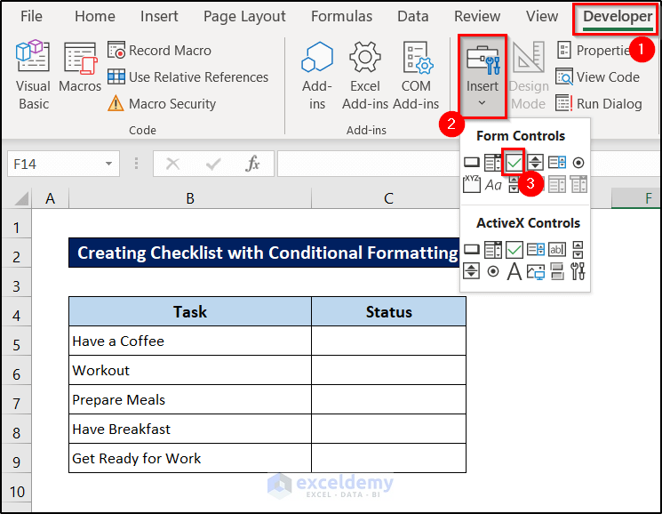
- Select the Check box (Form Control) from the drop-down menu.
- Place the box in its appropriate place.
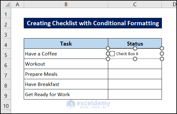
- Right-click on the box and select Format Control from the context menu.
- Go to the Control tab on the box and select cell C5 as its linked cell.
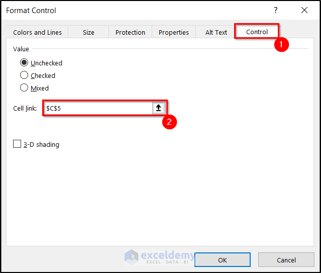
- Click on OK.
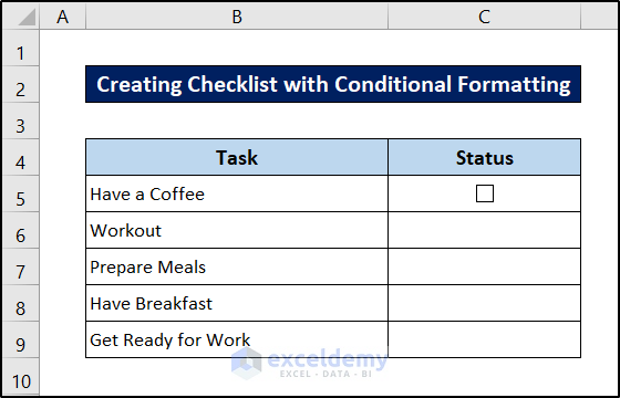
- Remove the alt text and place the checkbox in the middle of the cell.
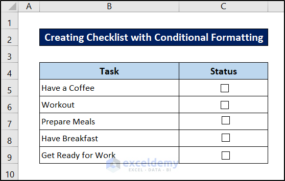
- Repeat the process for all of the boxes.
- Once checked, there will be a TRUE/FALSE value on the cells depending on it.
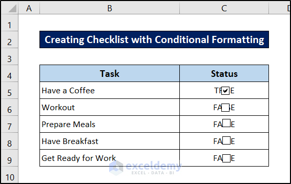
- Use a white font color to make them invisible.
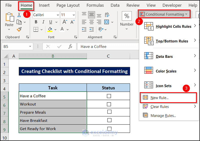
- Select the task range you want to format.
- Go to the Home tab on your ribbon.
- Select Conditional Formatting from the Styles group section.
- Select New Rule from the drop-down menu.
- In the Formatting Rule box, select the Use a formula to determine which cells to format option under Select a Rule Type.
- Insert the following formula in the Format values where this formula is true.
=C5=TRUE
- Select your preferred format type. We chose a strikethrough font.
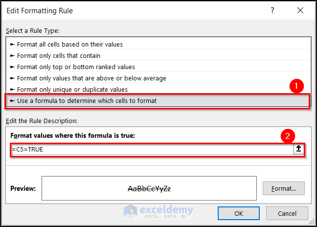
- Click on OK.
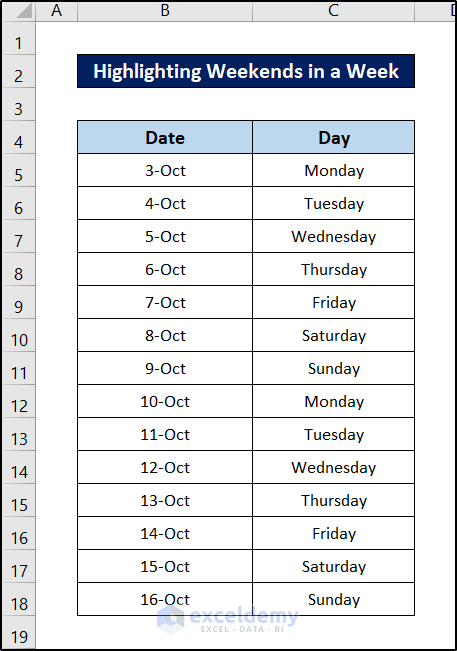
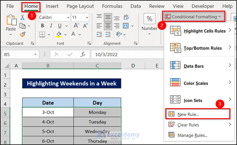
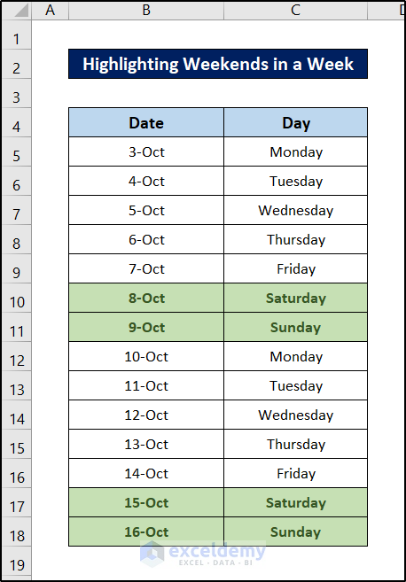
Example 21 – Highlight Weekends in a Week
We will use the OR and WEEKDAY functions to create this formula.
Steps:
- Select all the cells in the dataset excluding headers.
- Go to the Home tab on your ribbon.
- Select Conditional Formatting from the Styles group section.
- Select New Rule from the drop-down menu.
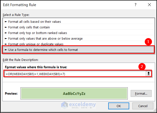
- In the Formatting Rule box, select the Use a formula to determine which cells to format option under Select a Rule Type.
- Insert the following formula in the Format values where this formula is true.
=OR(WEEKDAY($B5)=1,WEEKDAY($B5)=7)
- Select your preferred format type.
- Click on OK.
Download the Practice Workbook
Conditional Formatting with Formula in Excel: Knowledge Hub
- Format Cell Based on Formula
- Use Conditional Formatting Based on VLOOKUP
- Apply Conditional Formatting with INDEX-MATCH
- Excel Conditional Formatting Formula with IF
- Apply Conditional Formatting Formula in Excel If Cell Contains Text
<< Go Back to Conditional Formatting | Learn Excel
Get FREE Advanced Excel Exercises with Solutions!
