Conditional formatting allows you to change the appearance of cells based on specific criteria that you define. When the conditions are met, the cell range is formatted according to your specifications. Conversely, if the conditions are not satisfied, the cell range remains unformatted. While Excel provides several built-in conditions, you can also create custom rules.

In this example, we’ll compare two columns and use conditional formatting to highlight matching or duplicate values.

Method 1 – Compare Two Columns for Matching Values in the Same Row

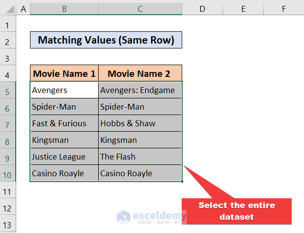
To demonstrate this, we are going to use this dataset:

Here, we have some movie names. Our goal is to compare two columns and highlight those rows having matching values.

Step-by-Step Guide

• Select the entire data range containing the two columns you want to compare. For instance, let’s say we have movie names in columns B and C (cells B5:C10).

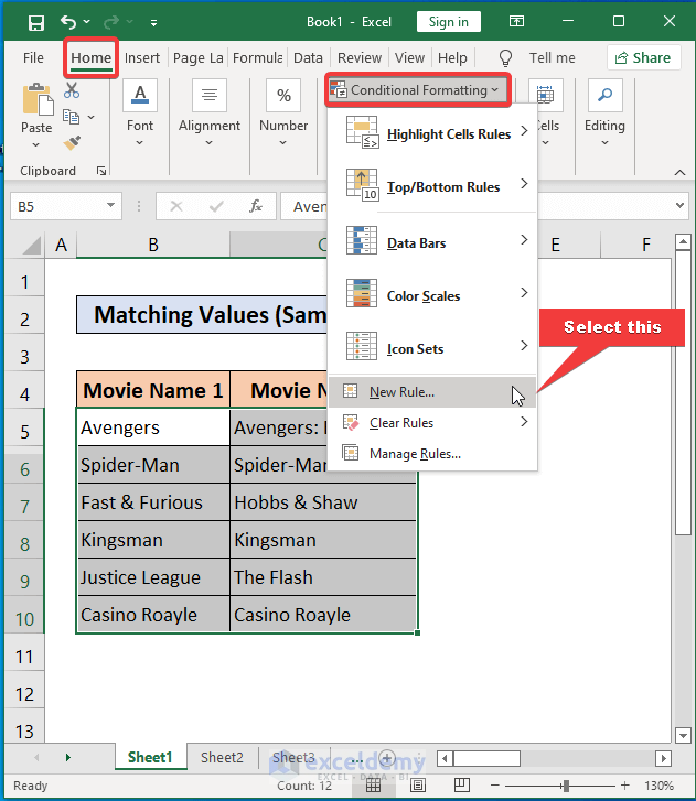
• Go to the Home tab in Excel.
• Click on Conditional Formatting and choose New Rule.

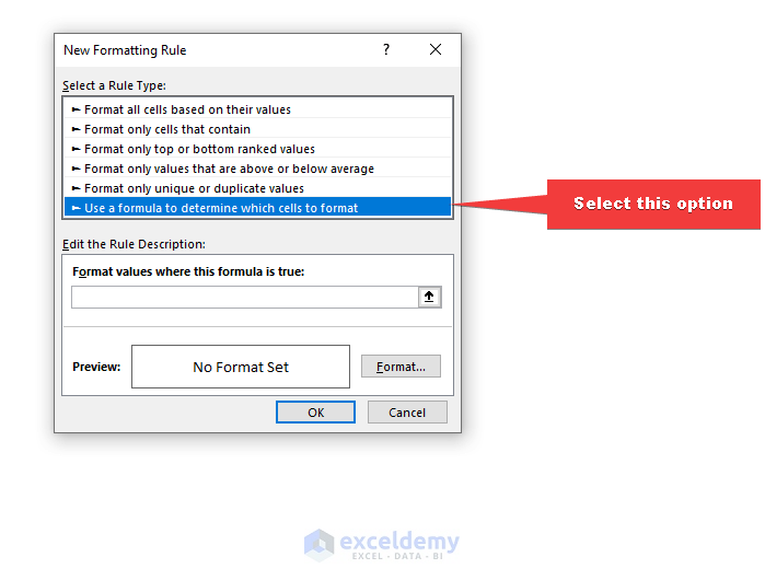
• In the New Formatting Rule dialog box, select Use a formula to determine which cells to format.

• In the Format values where this formula is true field, enter the following formula:

• • This formula checks if the value in column B (cell B5) is equal to the value in column C (cell C5) for each row.

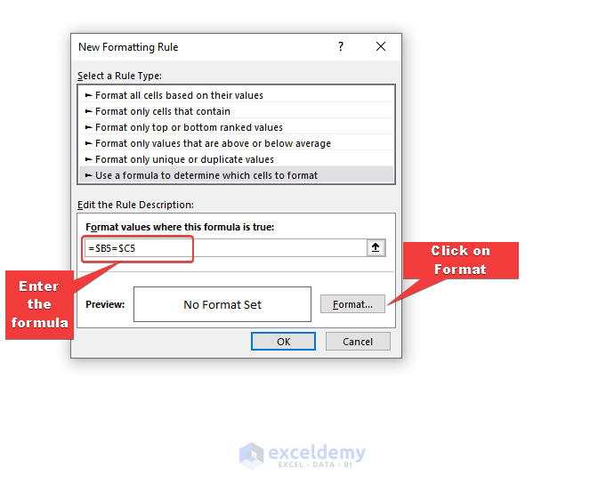
• Click on the Format button.
• In the Format Cells dialog box, navigate to the Fill tab.

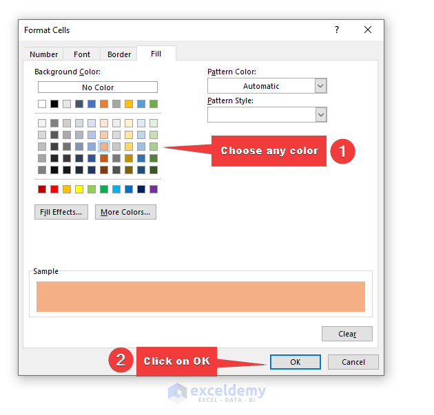
• Choose a suitable color to highlight the matching values (e.g., green) and click OK.

• Confirm the formula and formatting settings by clicking OK in the New Formatting Rule dialog box.

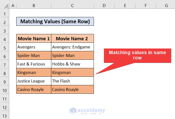
Now, your rows with matching data will be visually formatted according to your chosen color. You’ve successfully used conditional formatting to compare two columns in Excel!

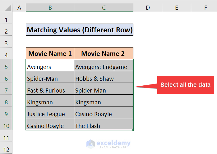
Method 2 – Use Conditional Formatting for Matching Values in Different Row in Excel

Sometimes, we encounter situations where the same values appear in two different columns but occupy different rows. In such cases, we want to compare these two columns and highlight any duplicate values using conditional formatting.

Here’s how you can achieve this:

Step-by-Step Guide

• Select the entire data range that includes the two columns you wish to compare. For instance, let’s assume we have movie names in columns B and C (cells B5:C10).

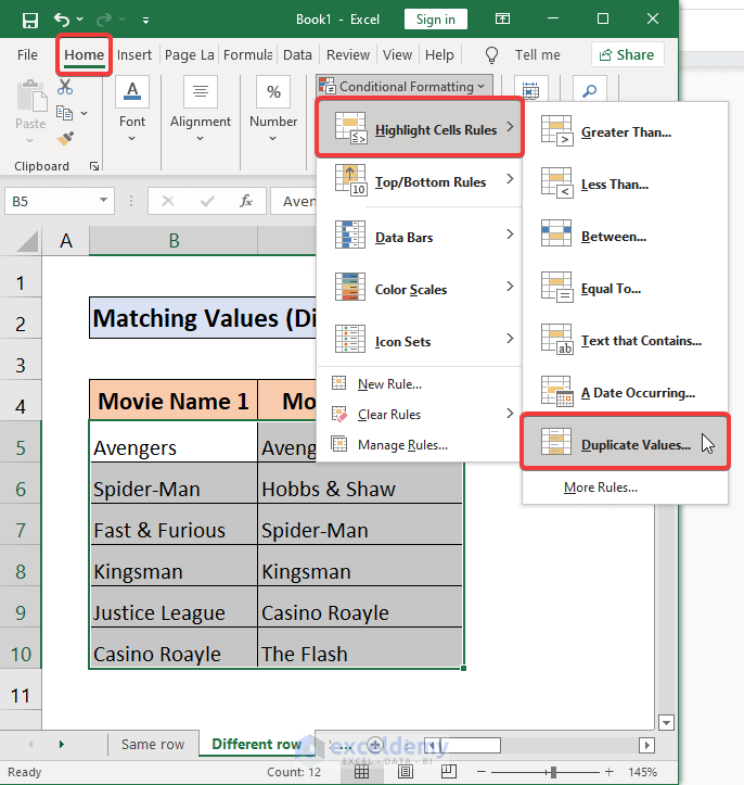
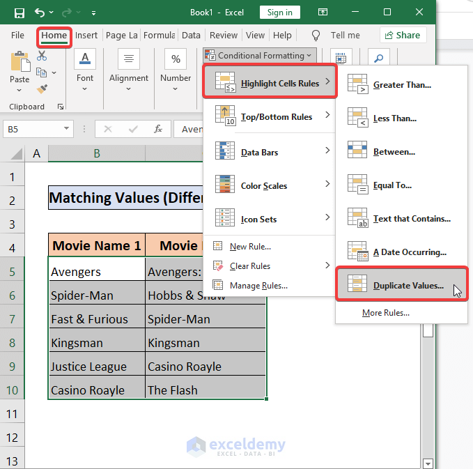
• Go to the Home tab in Excel.
• Click on Conditional Formatting and choose Highlight Cells Rules, then select Duplicate Values.

• In the Duplicate Values dialog box, you can pick any fill color to highlight the matching values. If you have specific preferences, use the Custom Format option to select your preferred colors.

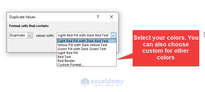
• Click OK to confirm your choices.

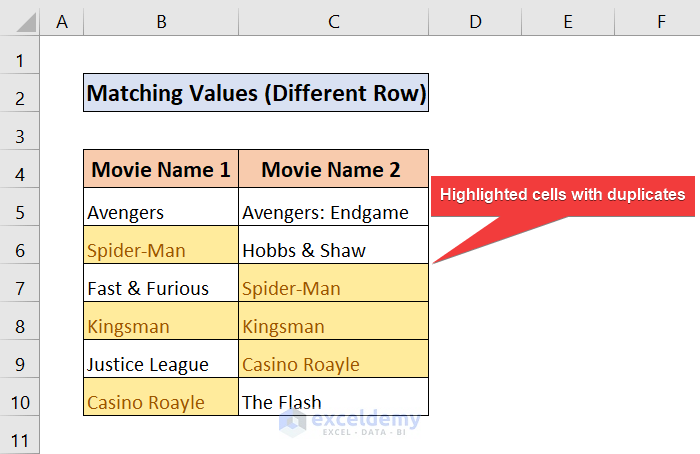
As a result, all matching values between the two columns will be visually highlighted. You’ve successfully used conditional formatting to identify duplicate values in different rows.

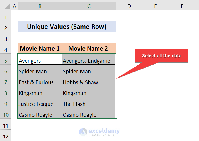
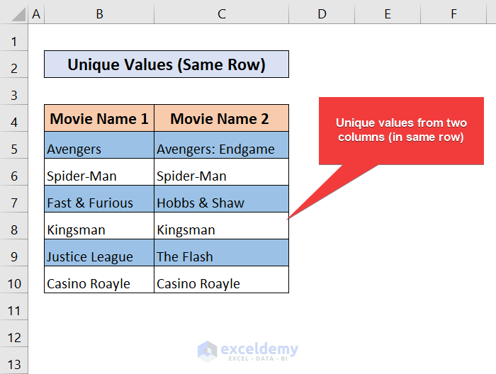
Method 3 – Use Conditional Formatting for Unique Values from Two Columns but the Same Row

Sometimes, you’ll encounter unique values in two different columns within the same row. To identify and highlight these unique values, we are going to use this dataset and follow these steps:

Step-by-Step Guide

• Select the entire dataset that includes the two columns you want to compare. For instance, let’s assume we have movie names in columns B and C (cells B5:C10).

• Go to the Home tab in Excel.
• Click on Conditional Formatting and choose New Rule.

• In the New Formatting Rule dialog box, select Use a formula to determine which cells to format.

• In the Format values where this formula is true field, enter the following formula:

• • This formula checks if the value in column B (cell B5) is different from the value in column C (cell C5) for each row.

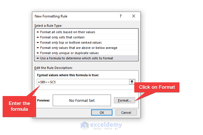
• Click on the Format button.
• In the Format Cells dialog box, navigate to the Fill tab.

• Choose any color you prefer to highlight the unique values (e.g., yellow) and click OK.

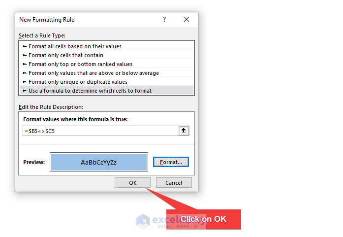
• Confirm the formula and formatting settings by clicking OK in the New Formatting Rule dialog box.

Now, your cells with unique data in the same row will be visually formatted according to your chosen color.

Method 4 – Compare Two Columns and Find Unique Values from Two Columns and Different Rows

To identify all unique values from two columns across all rows, we are going to use this dataset and follow these steps: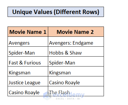

Step-by-Step Guide

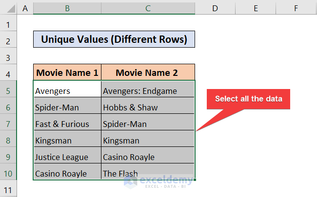
• Start by selecting the entire dataset.

• Go to the Home tab in Excel.
• Click on Conditional Formatting and choose Highlight Cells Rules, then select Duplicate Values.

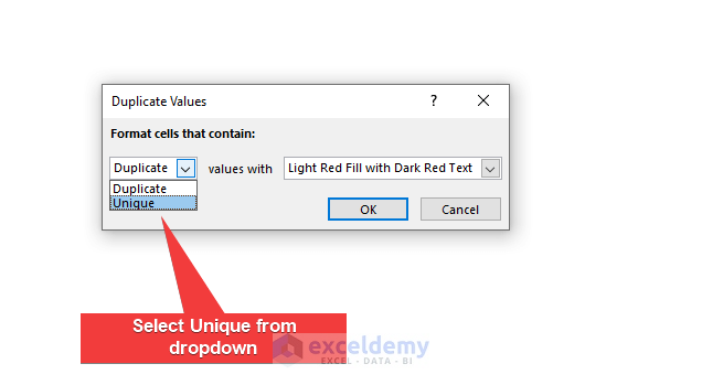
• In the Duplicate Values dialog box, select the Unique option from the drop-down menu.

• You can choose any fill color to highlight the unique values. If you have specific preferences, use the Custom Format option.

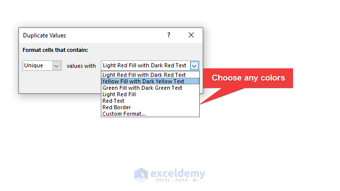
• Click OK to confirm your choices.

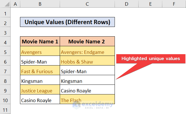
As a result, all unique values from the two columns will be visually highlighted across different rows. You’ve successfully used conditional formatting to find and emphasize unique data!

Compare Two Columns and Use Conditional Formatting for Greater or Less than a Value

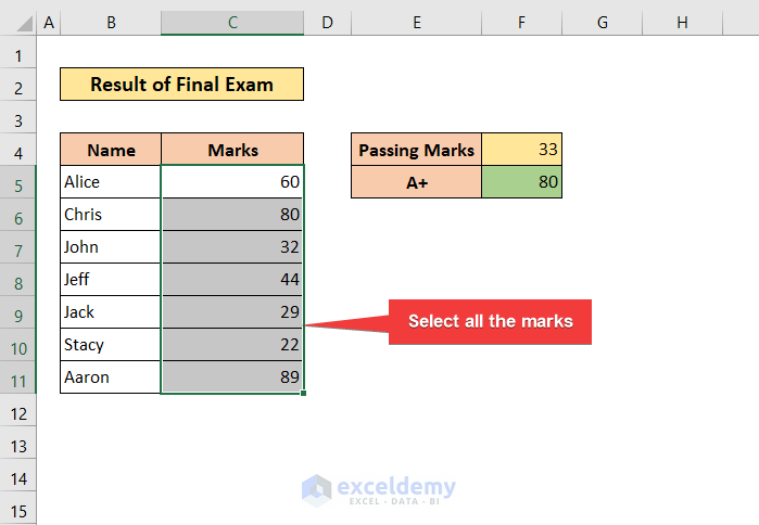
In this scenario, we’ll compare two columns that are not adjacent to each other. Specifically, we want to compare a column with a value from a different column. Let’s use the following dataset as an example:

• Dataset:
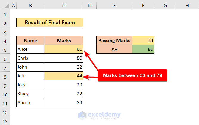
  • We have scores for some students.
  • The passing mark is 33.
  • To achieve an A+, students need to score 80 or higher.

Steps

• Select all the marks from your dataset.

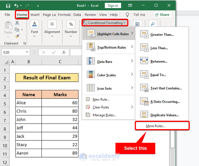
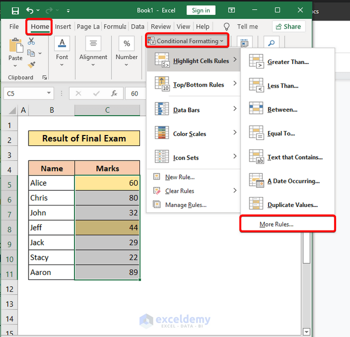
• Go to the Home tab in Excel.
• Click on Conditional Formatting and choose More Rules.

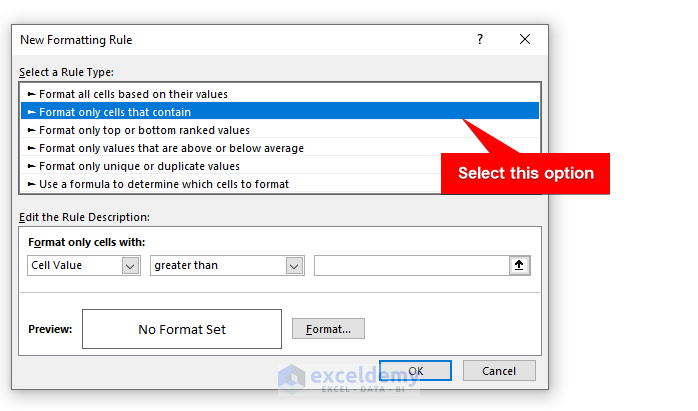
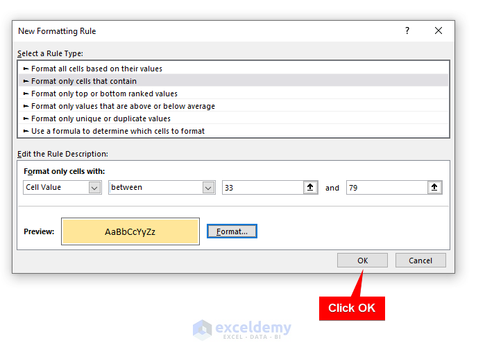
• In the New Formatting Rule dialog box, select Format only cells that contain.

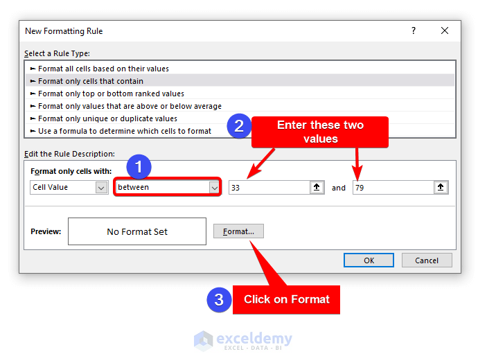
• Choose Between from the dropdown menu.
• Enter the values 33 and 79 (you can also use cell references).
• Click on Format.

• Choose a color (e.g., yellow) and click OK.

• Confirm your choices by clicking OK again.

You will see highlighted marks between 33 and 79.

• Select all the marks again.

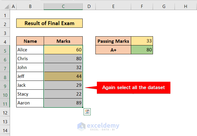
• Go to Conditional Formatting and select More Rules.

• Choose greater than or equal to from the dropdown menu.

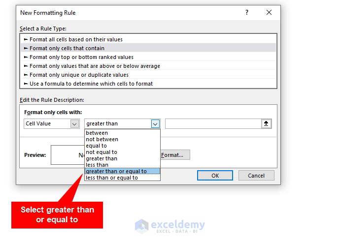
• Enter the value 80 (or use the cell reference for A+).
• Format the fill color as green.

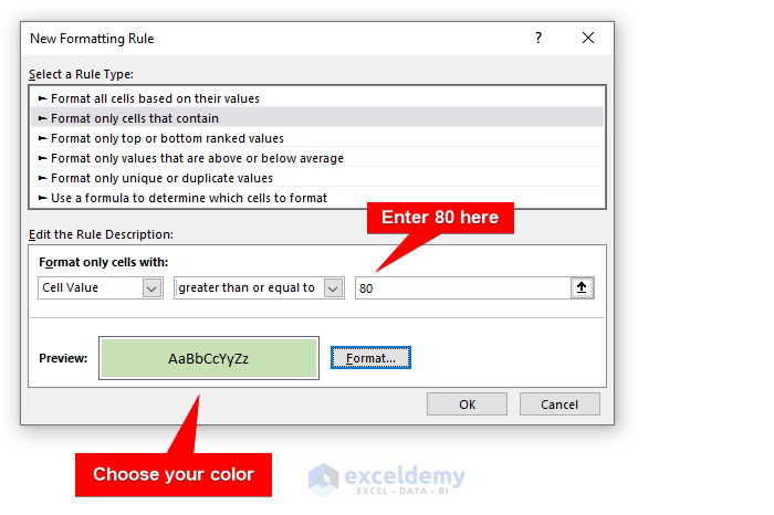
• • Click OK.

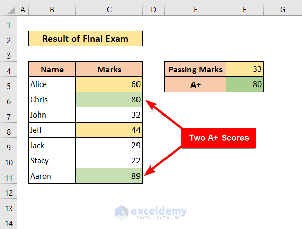
Now, your marks between 33 and 79 will be highlighted in yellow, and A+ scores (80 or more) will be highlighted in green. You’ve successfully used conditional formatting for different score ranges in Excel!

Additional Tips

• If you add new rows, remember to adjust the range for formatting rules.
• Be cautious when selecting cell ranges; incorrect choices can affect the behavior of conditional formatting.

Download Practice Workbook

You can download the practice workbook from here:

Further Readings

• How to Apply Different Types of Conditional Formatting in Excel
• How to Find External Links in Conditional Formatting in Excel
• How to Apply Conditional Formatting for Blank Cells in Excel
• How to Apply Conditional Formatting on Multiple Columns in Excel
  
• How to Remove Conditional Formatting in Excel
• How to Remove Conditional Formatting but Keep the Format in Excel
• How to Do Conditional Formatting in Excel
• Conditional Formatting with Formula in Excel

<< Go Back to Conditional Formatting | Learn Excel