⏷What Is Conditional Formatting in Excel?
⏷Where Is Conditional Formatting Located in Excel?
⏷Apply Different Types of Conditional Formatting
⏵Highlight Cells Rules
⏵Top/Bottom Rules
⏵Data Bars
⏵Color Scales
⏵Icon Sets
⏷Create a New Conditional Formatting Rule
⏷Edit Conditional Formatting Rules
⏷Copy Conditional Formatting
⏷Conditional Formatting with Single or Multiple New Rules
⏷Conditional Formatting Based on Another Cell
⏷Highlight Errors/Blanks
⏷Highlight Odd or Even Rows
⏷Highlight Every nth Row
⏷Dynamic Search for a Value and Highlight Corresponding Cells
⏷Find Cells with Conditional Formatting
⏷Remove Conditional Formatting in Excel
What Is Conditional Formatting in Excel?
Conditional formatting is a technique that allows you to modify cell formatting based on specific conditions. For instance, if you have an Excel worksheet with numerical values, you can apply formatting rules to highlight cells with values less than three thousand. In this case, the condition is that the numbers must be less than three thousand, and the desired formatting is a red background.
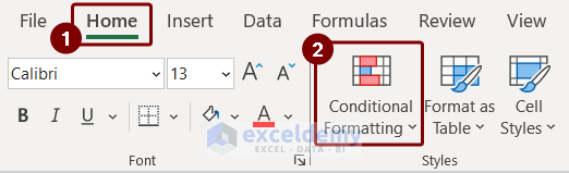
Where Is Conditional Formatting Located in Excel?
You can access conditional formatting through the Styles section on the Home tab of the Ribbon.
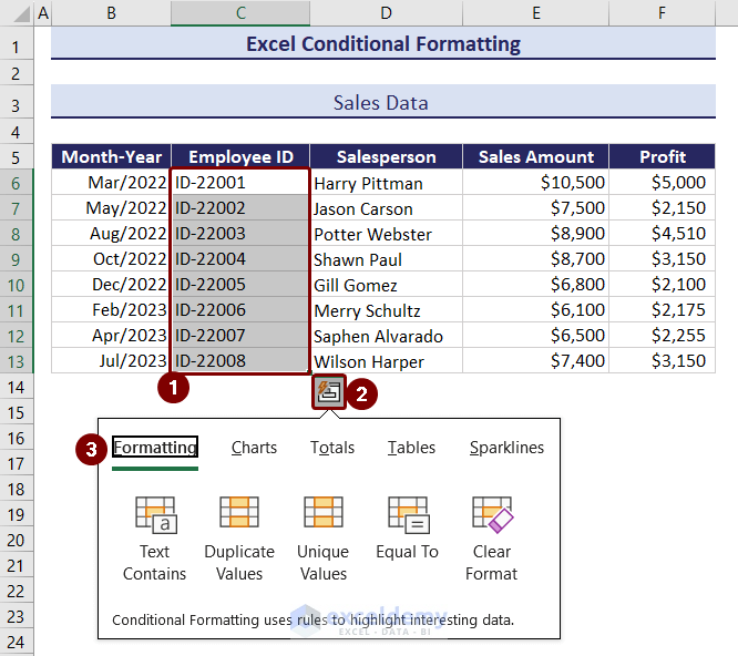
Additionally, a quicker way to apply conditional formatting is via the Quick Analysis Tool, which appears at the bottom-right corner of any selected range in the worksheet.
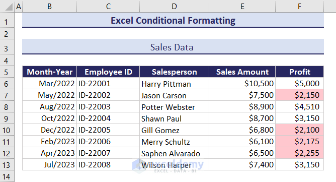
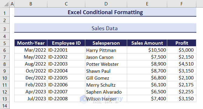
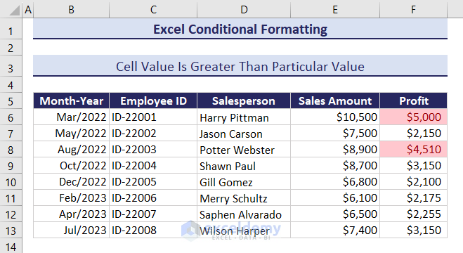
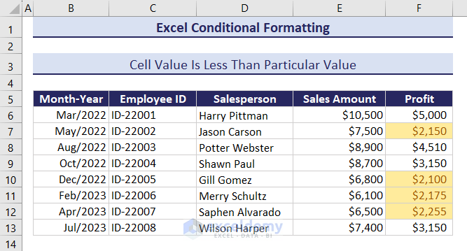
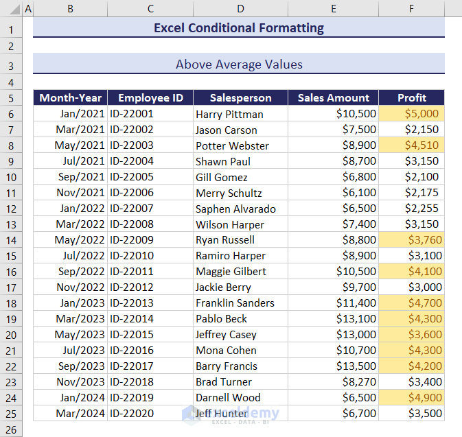
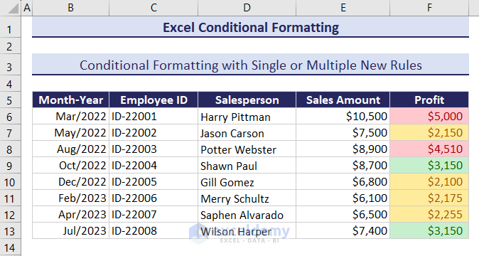
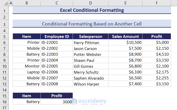
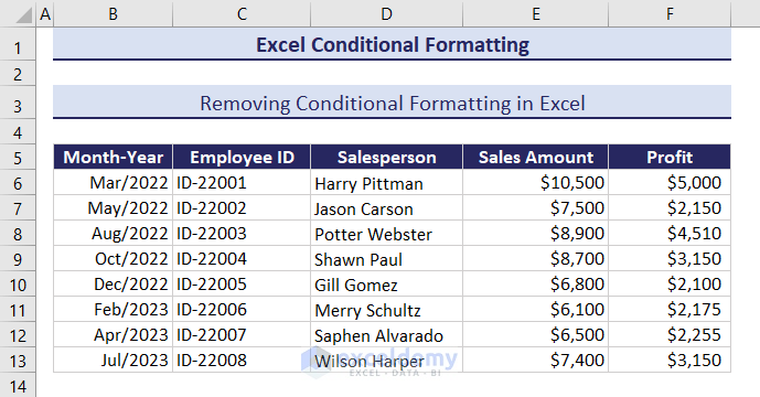
Dataset Overview
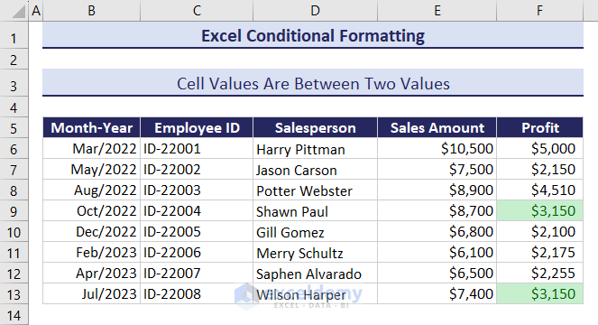
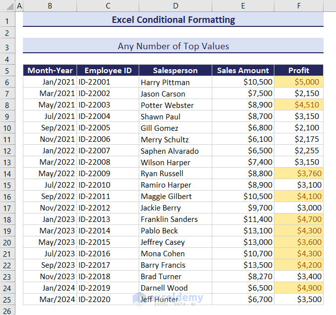
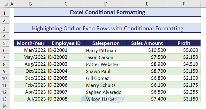
Let’s explore various types of conditional formatting available in Excel on the Windows operating system. I’ll use a sample dataset for illustration, where column B contains month values, column C has employee IDs, column D lists salesperson names, column E shows sales amounts, and column F displays earned profit for a specific month. Based on different criteria, we’ll apply formatting rules to this dataset.
1. Highlight Cells Rules
You can highlight cells based on specific rules, such as greater than, lesser than, or within a certain range. Let’s start with an example:
Criteria 1: Cell Value Is Greater Than Particular Value
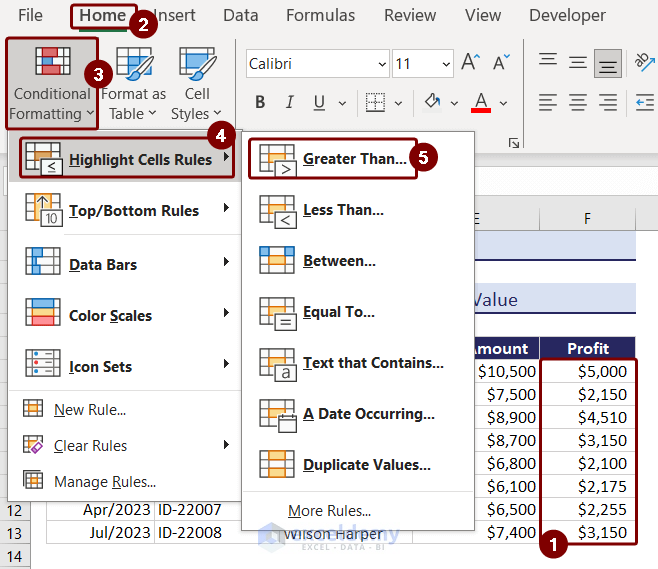
- Select the cell range F6:F13.
- Go to the Home tab, click on Conditional Formatting, and choose Highlight Cells Rules.
- From the dropdown menu, select Greater Than.
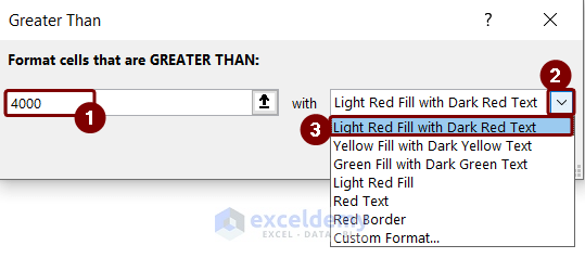
- Set the comparison value to 4000.
- Choose a light red fill with dark red text format.
- Click OK to apply the formatting.
- The result will look like the image below.
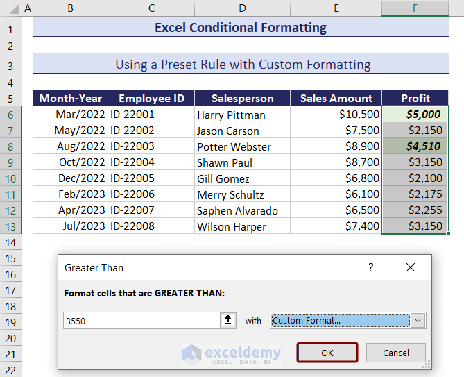
Using a Preset Rule with Custom Formatting
- Select the same cell range (F6:F13).
- Go to Home > Conditional Formatting > Highlight Cell Rules > Greater Than.
- In the Greater Than dialog box, enter 3550 as the comparison value.
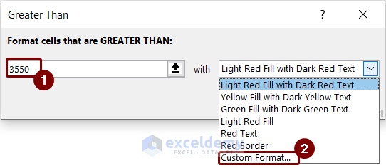
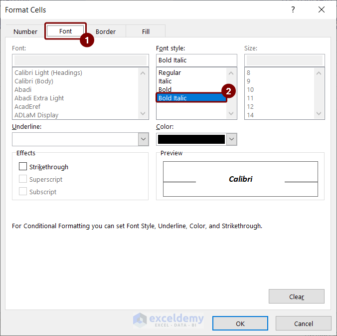
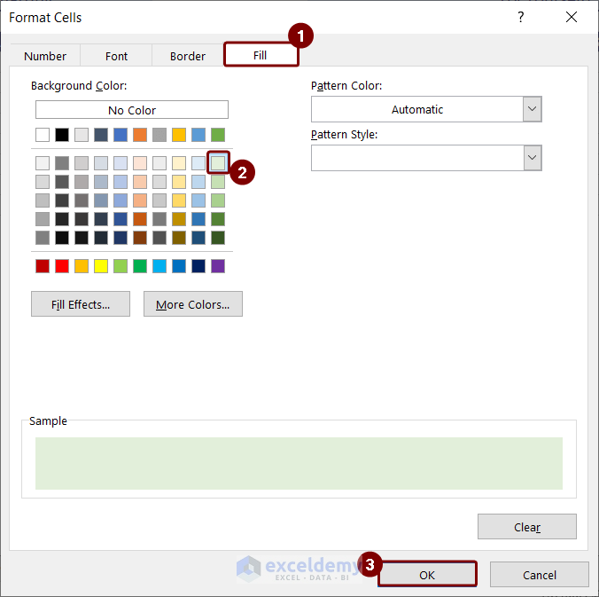
- Choose custom formatting: bold italic font and light green fill color.
- Confirm by pressing OK.
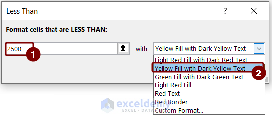
Criteria 2: Cell Value Is Less Than Particular Value
- Select the cell range where you want to apply this rule.
- Go to Highlight Cells Rules and select Less Than.
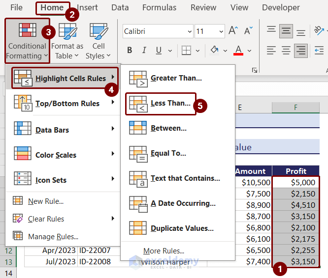
- Set the comparison value to 2500.
- Apply yellow fill with dark yellow text formatting.
- Press OK to close the dialog box.
- This is the output after the conditional formatting is applied.
Criteria 3: Cell Values Are Between Two Values
In this case, we want to highlight cells with values falling between two specified thresholds. Follow these steps:
- Select the cell range (F6:F13).
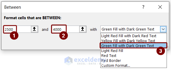
- Go to Conditional Formatting and choose Between.
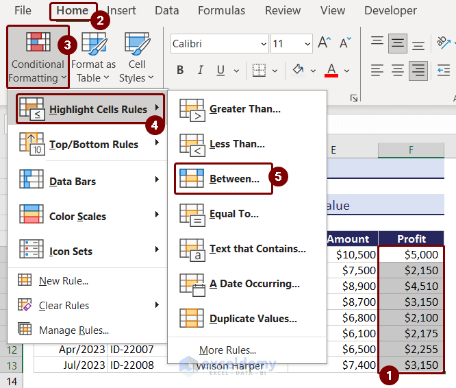
- Set the range values (e.g., 3000 and 4500).
- Apply a green fill with dark green text.
- Press OK to apply the formatting.
- Herewith the output after the conditional formatting is applied.
Criteria 4: Cell Value Is Equal to Particular Value
To highlight cells equal to a specific value:
- Select the cell range (F6:F13).
- Choose Equal To from the Highlight Cells Rules.
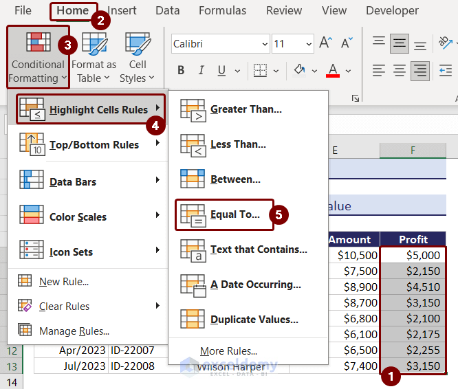
- Set the value (e.g., 2100).
- Apply a light red fill.
- Cell F10 will be highlighted.

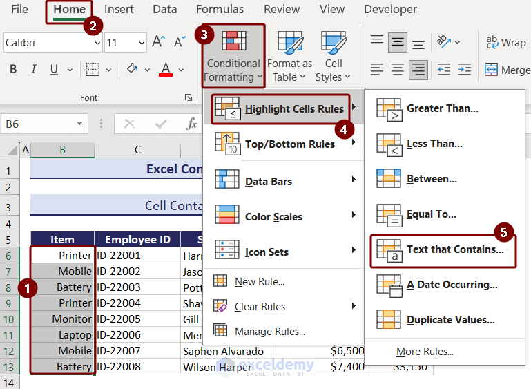
Criteria 5: Cell Containing Particular Text
This condition focuses on text-based highlighting:
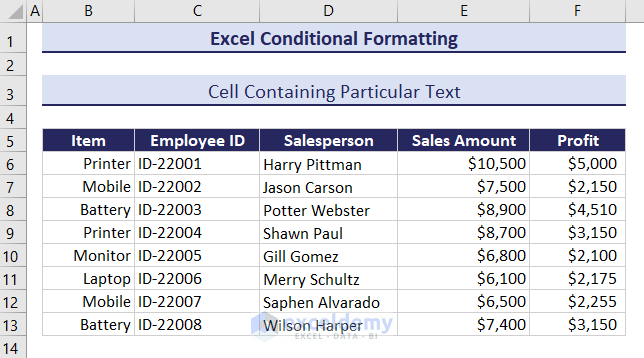
- Select the cell range (B6:B13).
- Use Text that Contains from the Highlight Cells Rules.
Click the image to get a better view
- In the dialog box, type Printer.
- Apply a light red fill with dark red text.
- Press OK to close the box.

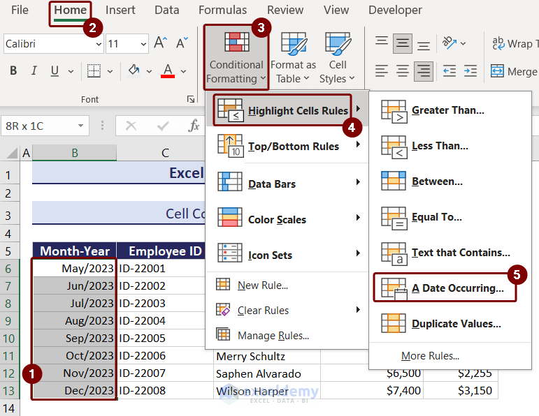
Criteria 6: Cell Containing Particular Dates
For date-based formatting:
- Select the cell range containing dates (B6:B13).
- Choose A Date Occurring from the dropdown.
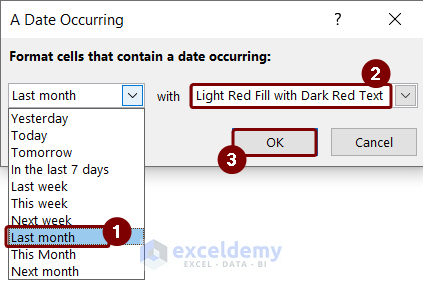
Click the image to get a better view
- Set the rule (e.g., Last month).
- Apply a light red fill with dark red text.
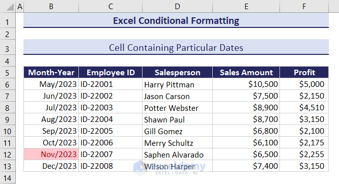
- As a result, in cell range B6:B13, only the previous month’s dates will be highlighted.
- Herewith the output after the conditional formatting is applied.
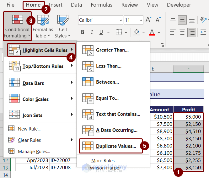
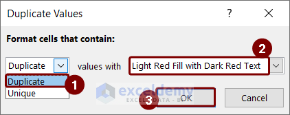
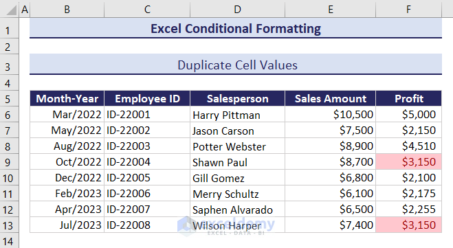
Criteria 7: Duplicate Cell Values
To find and highlight duplicates:
- Select the relevant cell range.
- Pick Duplicate Values from the dropdown.
- Opt for the Duplicate option.
- You can also highlight unique values by choosing Unique.
- The conditional formatting is applied to duplicate values.
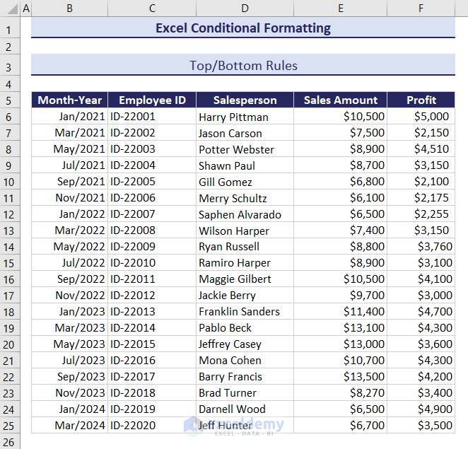
2. Top/ Bottom Rules
The Top and Bottom Rules represent the second type of Conditional Formatting in Excel. These rules allow you to highlight either the highest or lowest values from a large dataset or determine the top or bottom percentage of data. Let’s explore various scenarios using the dataset provided:
Case 1: Any Number of Top Values from the Data Set
- Select the cell range F6:F25.
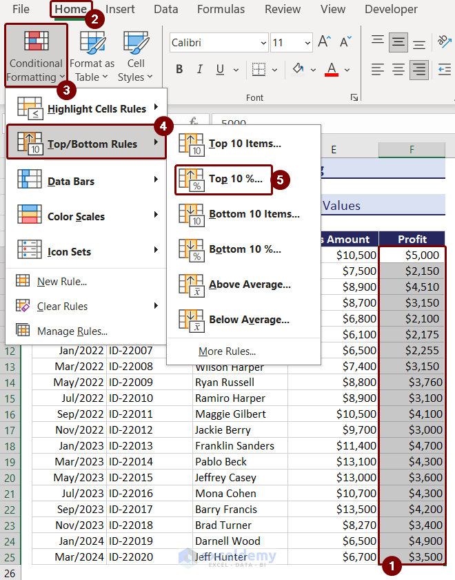
- Go to the Home tab and choose the Top/Bottom Rules option.
- From the rules, select Top 10 Items.
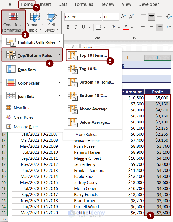
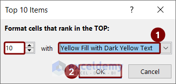
- A dialog box will appear where you can manually input the number of top values. Generally, it defaults to 10 if you have more than 10 values.
- Choose your desired formatting and press OK.
- This is the output after the conditional formatting is applied.
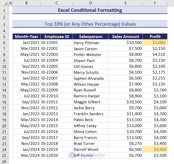
Case 2: Top 10% (or Any Other Percentage) of Values from the Data Set
- Select the cell range F6:F25.
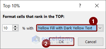
- Choose the Top 10% from the Top/Bottom Rules dropdown.
- Set the highlight condition as 10% and format the cells with Yellow Fill and Dark Yellow Text.
- Top 10% value will be highlighted.
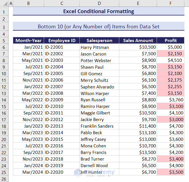
Case 3: Bottom 10 (or Any Number of) Items from the Data Set
- Select the data range F6:F25.
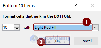
- Choose the Bottom 10 Items from the dropdown.
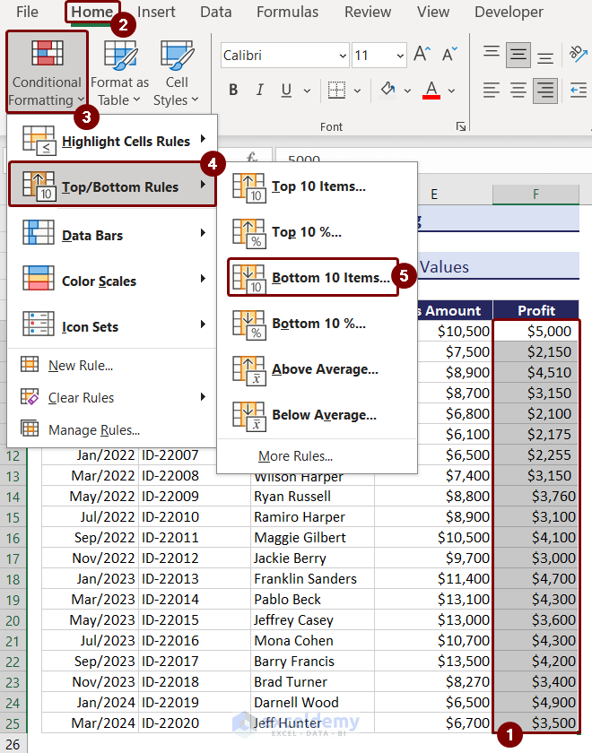
- Apply the desired formatting (format only) and press OK.
- The bottom 10 items are highlighted.
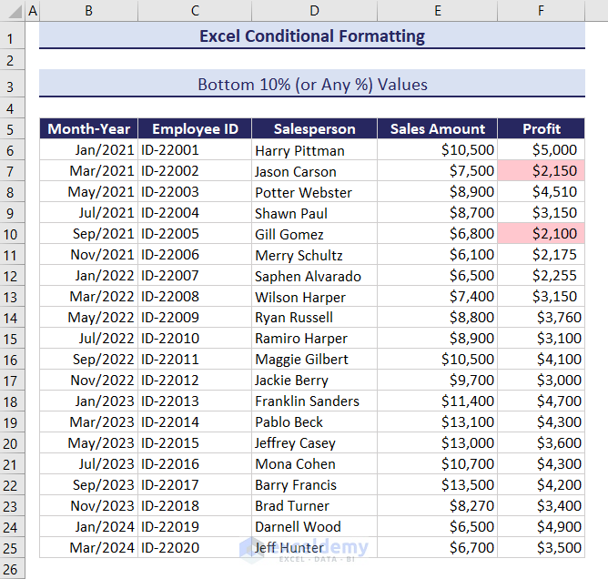
Case 4: Bottom 10% (or Any %) of Values from the Data Set
- Select the cells F6:F25.
- Go to the Top/Bottom Rules dropdown and choose Bottom 10%.
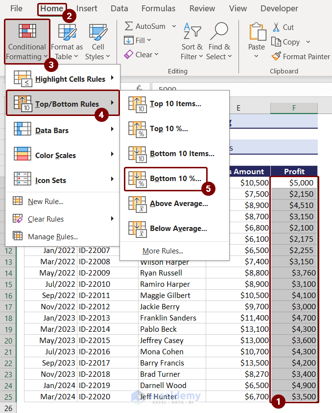
- Apply your preferred formatting and confirm.
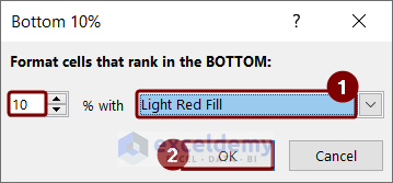
- The bottom 10% values will be highlighted.
Case 5: Above Average Values of the Data Set
- Select the cell range F6:F25.
- Use the Above Average condition from the Top/Bottom Rules.
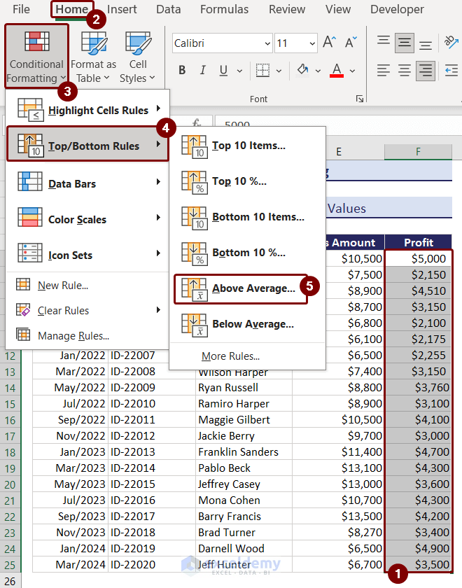
- Apply Yellow Fill with Dark Yellow Text formatting.
- Press OK.
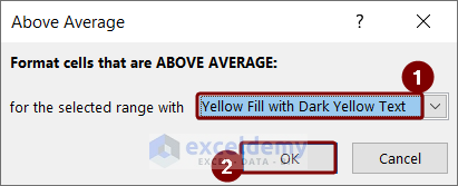
- The above-average values of the dataset are highlighted.
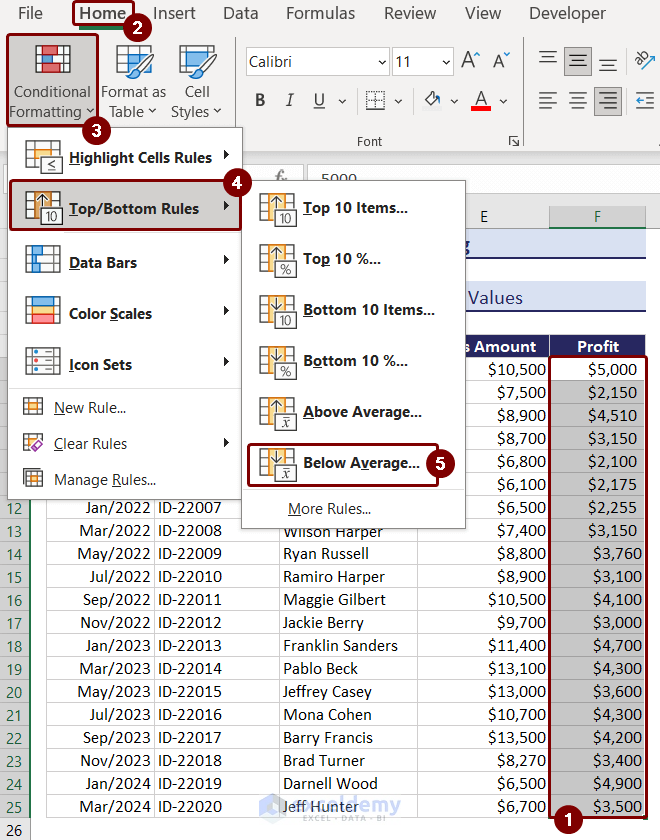
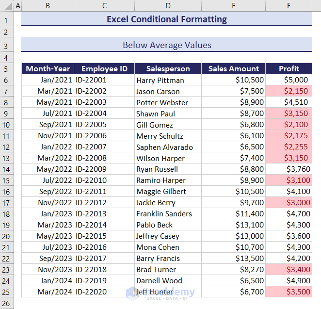
Case 6: Below Average Values of the Data Set
- Select cell range F6:F25.
- Choose Below Average from the dropdown.
- Format the cells with Light Red Fill and Dark Red Text.
- Press OK.
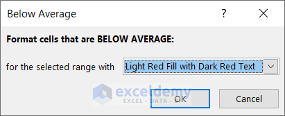
- The below-average values of the dataset are highlighted.
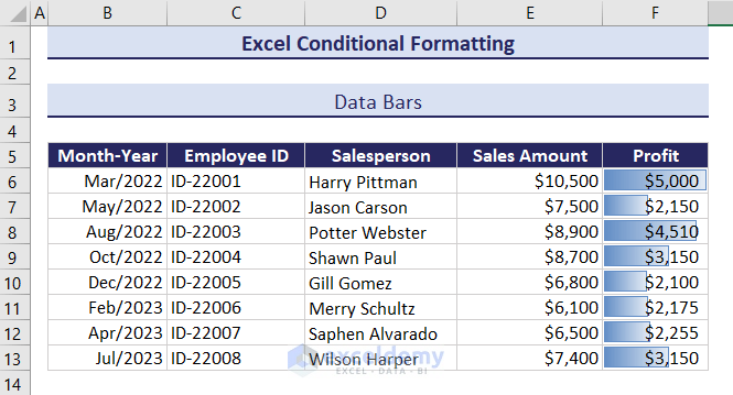
3. Data Bars
Data Bars represent the third type of conditional formatting in Excel. They visually display the distribution of values within a dataset. Let’s explore how to use data bars to show profit distribution:
- Select the cell range F6:F13.
- Go to the Home tab, click on Conditional Formatting, and choose Data Bars.
- Pick the Blue Data Bar or any other color scheme you prefer.
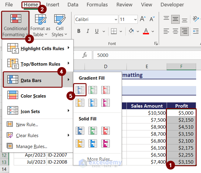
- The data bars will be added to the selected cells, visually representing the data distribution.
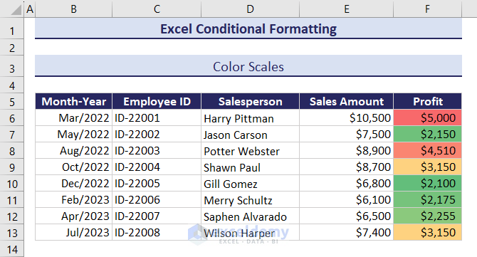
4. Color Scales
Color Scales are the fourth type of conditional formatting. They provide a visual representation of data disposal within a dataset. You can mix two or three colors on the scale. Here’s how to apply color scales:
- Select cell range F6:F13.
- From the Conditional Formatting dropdown, choose Color Scales.
- You’ll see various preexisting color sets for this condition.
- Select the Red-Yellow-Green color scale.
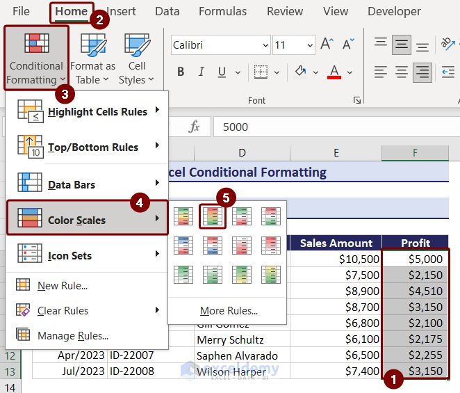
- The column will be formatted with different colors—red for lower values, yellow for average values, and green for higher values—based on increasing value.
If needed, you can customize the color scale further using the More Rules option.
5. Icon Sets
Icon Sets are the fifth type of conditional formatting. They work similarly to the previous examples, using icons based on cell values. Follow these steps:
- Choose the Icon Sets command from the “Conditional Formatting” dropdown, focusing on the cell range F6:F13.
- Select the 3 Triangle option from the directional icon sets.
![]()
- In this set, red icons represent lower values, yellow icons represent middle values, and green icons represent higher values in the dataset.
![]()
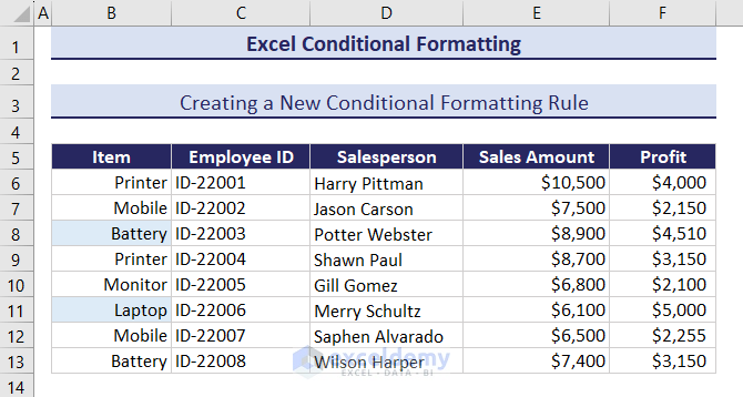
Creating a New Conditional Formatting Rule
Now, let’s apply conditional formatting using an INDEX-MATCH formula to find items with profit values greater than those of the printer:
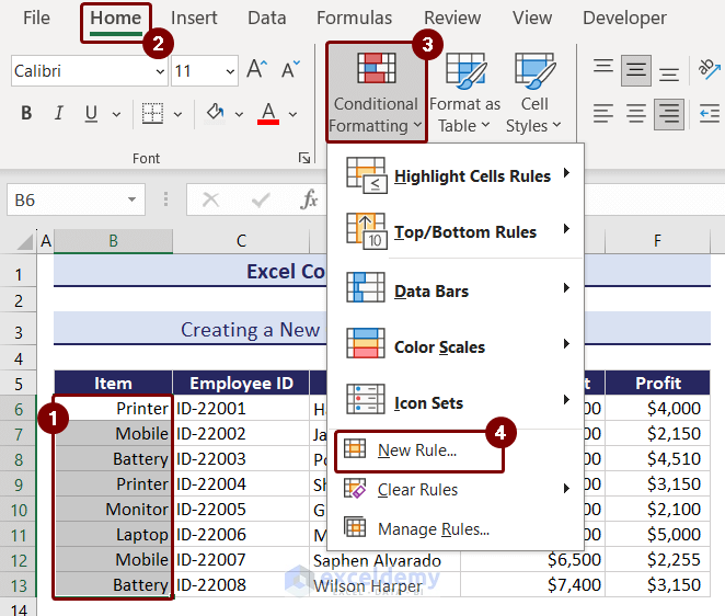
- Select the range B6:B13.
- Go to the Home tab, choose Conditional Formatting, and click New Rule.
- Alternatively, use the keyboard shortcut Alt + O + D.
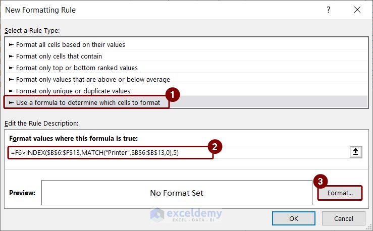
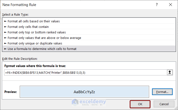
- In the New Formatting Rule box, select Use a formula to determine which cells to format.
- Insert the formula in the Format values where this formula is true section:
=F6>INDEX($B$6:$F$13,MATCH("Printer",$B$6:$B$13,0),5)- Press the Format button.
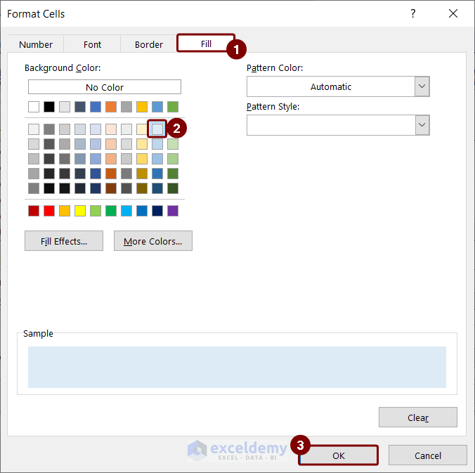
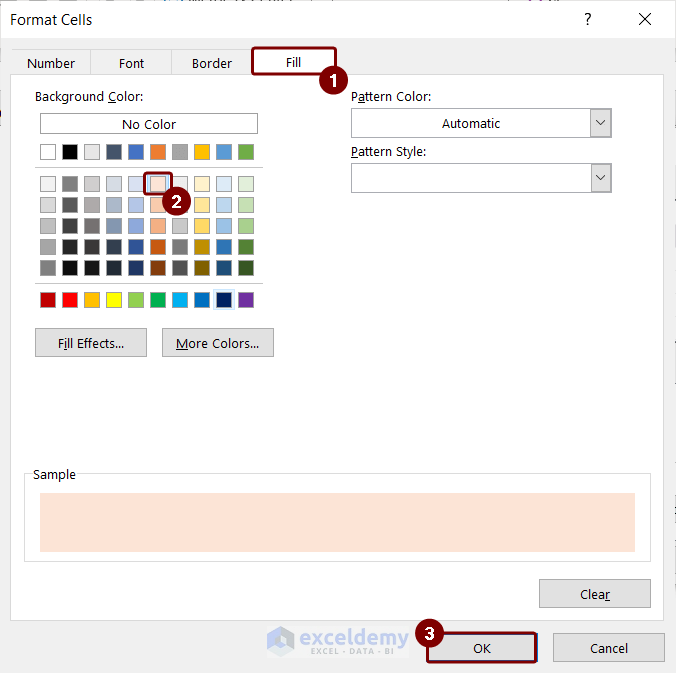
- In the Format Cells box, select the fill color you prefer and press OK
- New Formatting Rule box will appear again.
- Review the formula and formatting, then press OK.
- The items with greater profit values than printers will be highlighted.
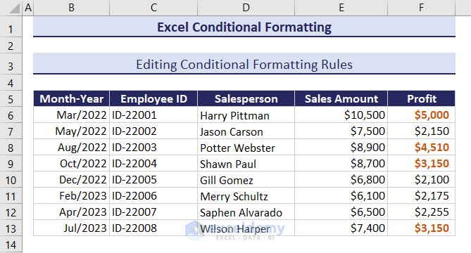
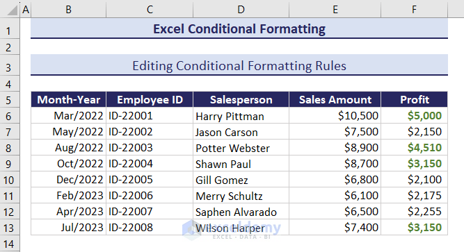
Editing Excel Conditional Formatting Rules
Let’s change the conditional formatting applied to cells F6:F13. Currently, they are formatted with the rule Cell Value > 3000 and an orange font color. We’ll change the text font color to green by editing the rule:
- Select cells F6:F13.
- Click on Home, select Conditional Formatting and click on Manage Rules.
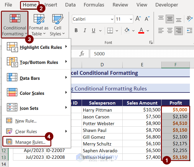
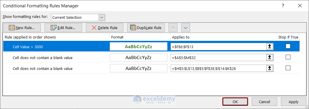
- The Conditional Formatting Rules Manager box will open.
- Select the rule and click Edit Rule.
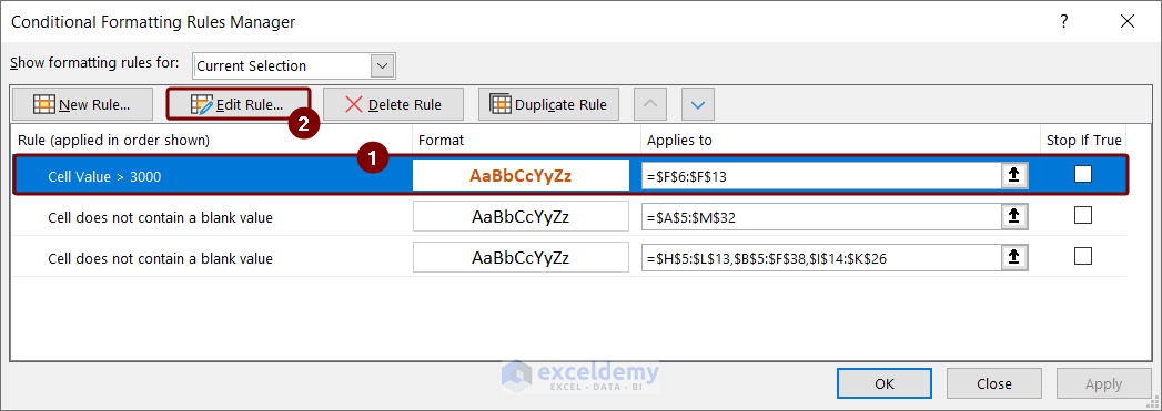
Click the image to get a better view
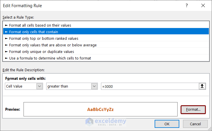
- In Edit Formatting Rule box, you will see the rule description.
- To change the formatting, press Format.
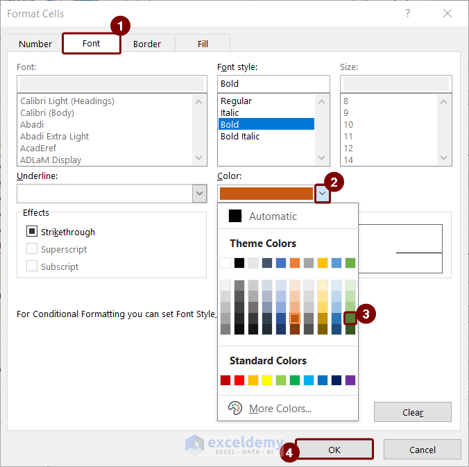
- In the Format Cells box, select the Font, click the Color drop-down, choose green, and press OK.
You can also adjust other formatting options (number type, font style, border, fill color) for the selected cells.
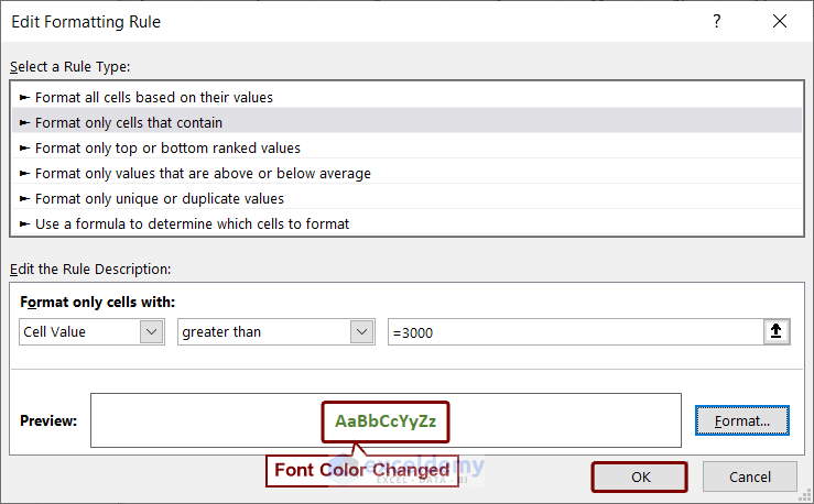
- Preview the font color change in the Edit Formatting Rule box and press OK.
- Confirm by pressing OK again in the Conditional Formatting Rules Manager.
Click the image to get a better view
The font color will now be green.
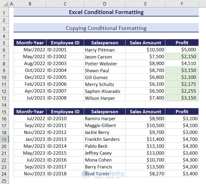
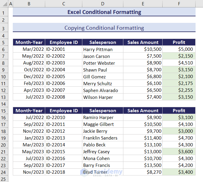
How to Copy Conditional Formatting
To copy the conditional formatting rule applied to the range F6:F13 into the range F16:F24, follow these steps:
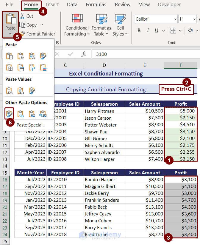
- Select the range F6:F13 and press Ctrl+C to copy.
- Select the range F16:F24 where we want to apply the formatting.
- Go to the Home tab, click the Paste drop-down, and choose Formatting from the Other Paste Options.
- As a result, the cell values between 2000 and 4000 will be highlighted with a light green color in the range F16:F24.
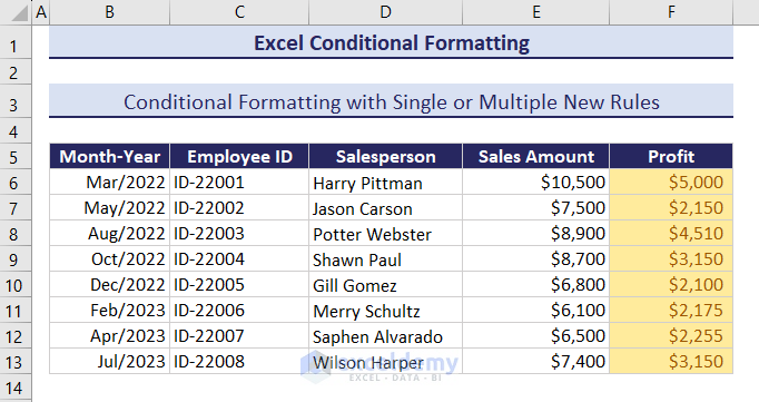
Conditional Formatting with Single or Multiple New Rules
Suppose you want to format multiple rules for the same dataset. While some rules won’t conflict, others might. For example:
- Green color if the cell value > 3500
- Yellow color if the cell values are between 2000 and 3500
- Red color if the cell values < 2000
However, consider the following conflicting rules:
- Green color if the cell value is > 3500
- Yellow color if the cell value is > 3000
- Red color if the cell value is > 2000
In this case, a number greater than 4000 satisfies both the yellow and green conditions, leading to a conflict. To address this, create a series of rules and apply the Stop if True condition.
✅ Managing Multiple Conditional Formatting Rules in the Same Dataset
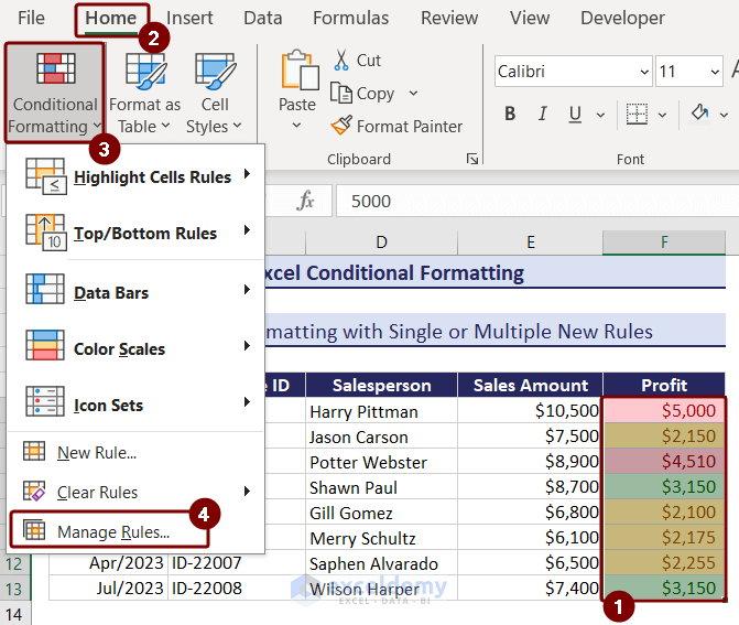
To organize conditional formatting rules for the same data, follow these steps:
- Select the column where the conditions apply.
- Go to the Home tab, select Conditional Formatting and click on Manage Rules.
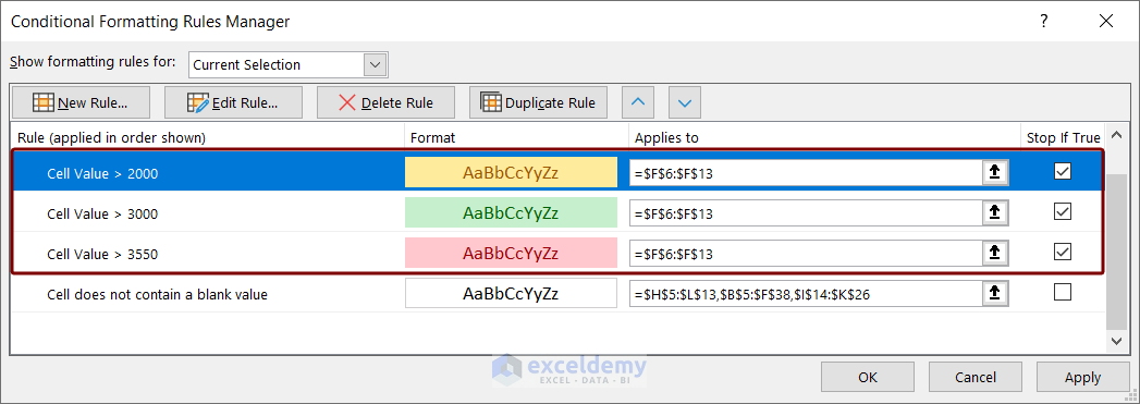
- In the Conditional Formatting Rules Manage” window, rules are listed in a specific order.
- Use the arrow buttons to sort the rules logically.
- Ensure that the Stop If True checkboxes are marked to apply rules correctly.
- By doing so, you’ll achieve the desired output.
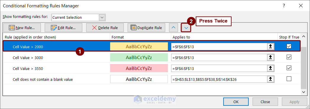
Click the image to get a better view
- If you unmark the checkboxes, then the output would be different.
- So, to get the desired result, we need to sort the rules. The first rule to check need to be Cell Value>3500. So, select the rule Cell Value>2000, and press the downside arrow button twice to transfer it.
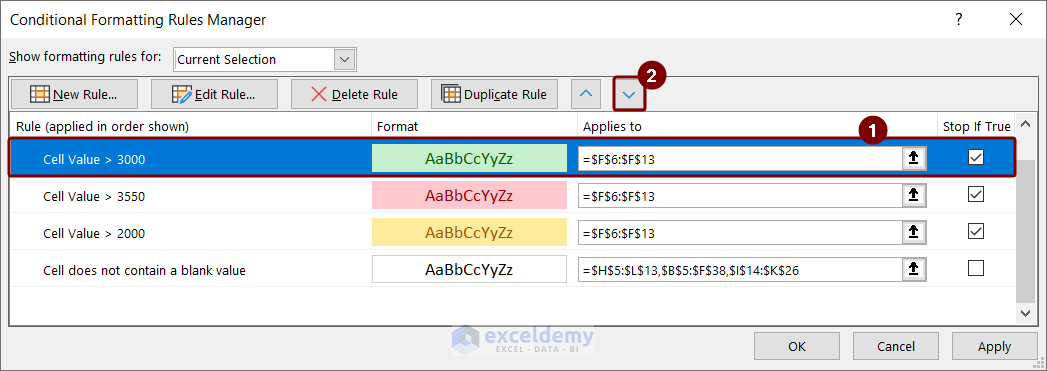
Click the image to get a better view
- Select Cell Value > 3000 rule and press the down button and you will have the rules in logical order.
Click the image to get a better view
- Keep the Stop If True checkboxes marked to ensure the proper application of the rules.
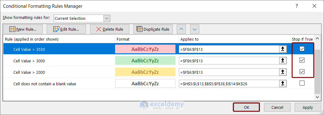
Click the image to get a better view
- Now, after sorting the rules, you will get the desired outcome.
Read More: Applying Conditional Formatting for Multiple Conditions in Excel
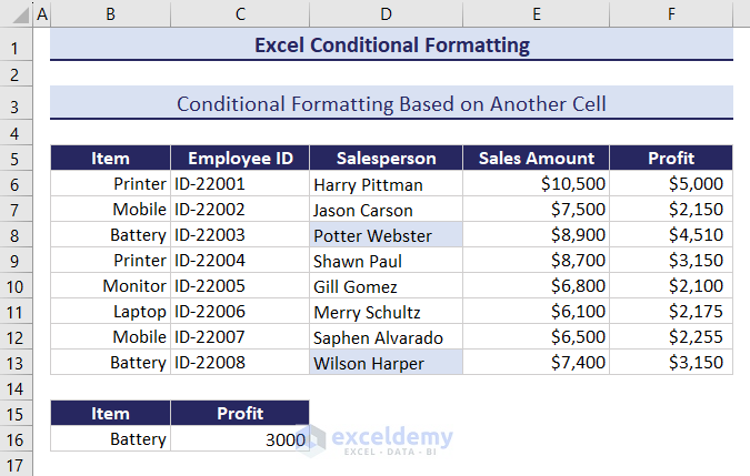
How to Do Conditional Formatting Based on Another Cell
You can create conditional formatting based on another cell or range. Let’s highlight salespeople who sold batteries and made a profit of $3000:
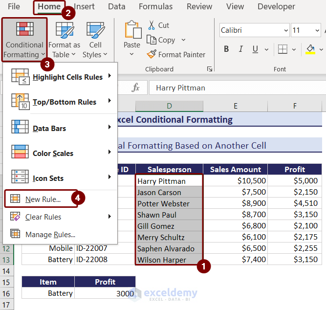
- Select cells D6:D13.
- Go to the New Rule option in Conditional Formatting.
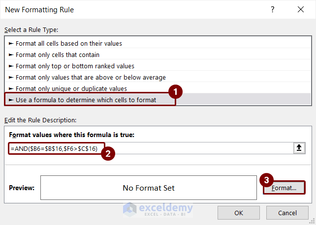
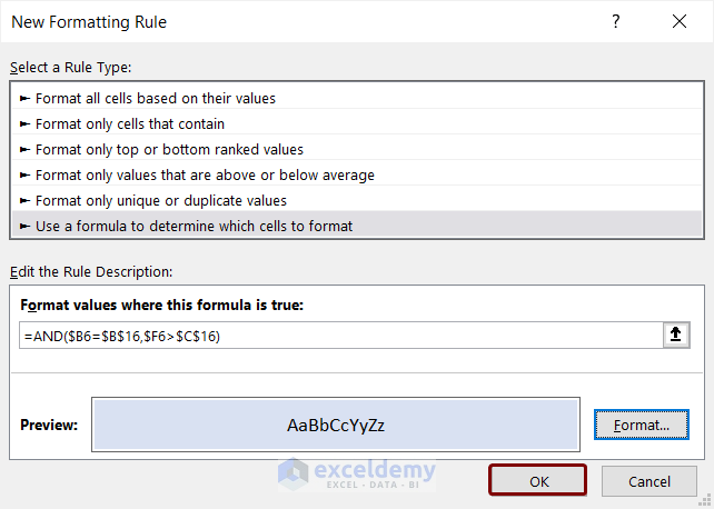
- Choose Use a Formula to determine which cells to format.
- Paste the following formula into the box:
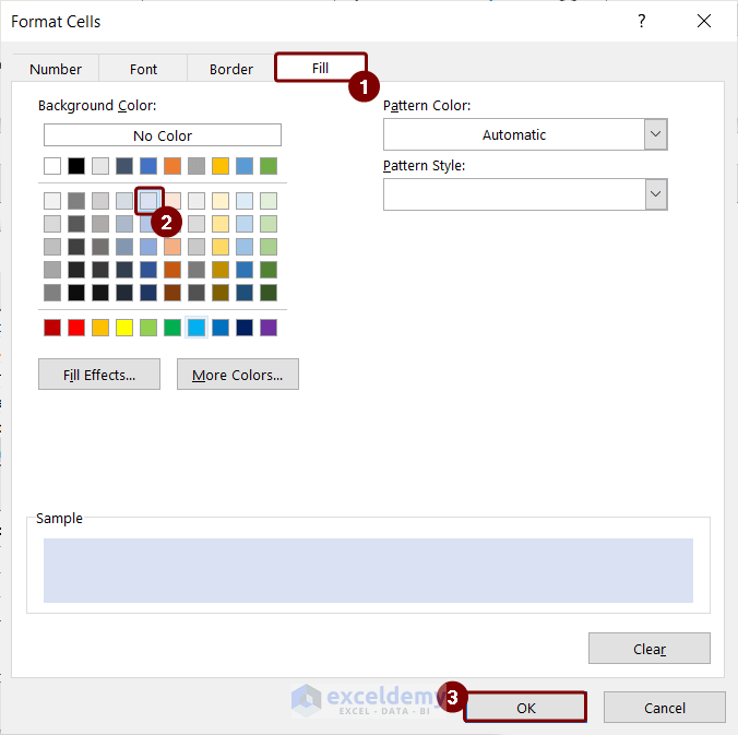
=AND($B6=$B$16,$F6>$C$16)- Click the Format button.
- Select a fill color for highlighting and press OK.
- Confirm the formatting rule.
- As a result, the Salesrep column cells corresponding to the Battery item with a profit greater than $3000 will be highlighted.
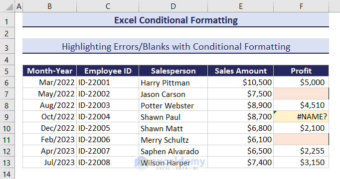
Highlighting Errors/Blanks with Conditional Formatting
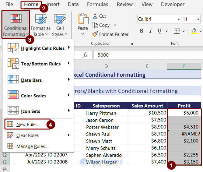
- Select the range F6:F13.
- Go to the Home tab in the Excel ribbon.
- Click on Conditional Formatting and choose New Rule from the dropdown.
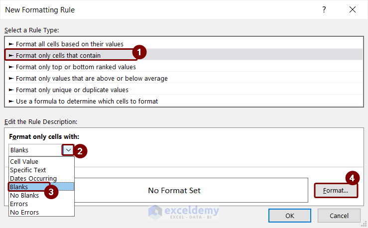
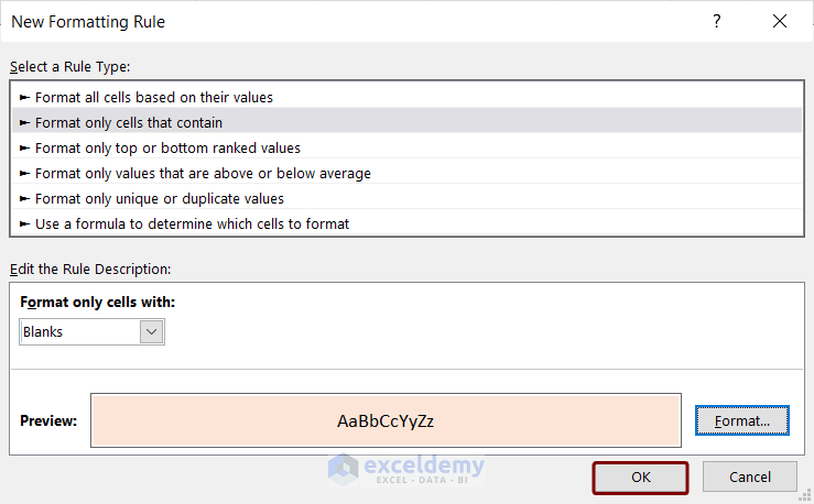
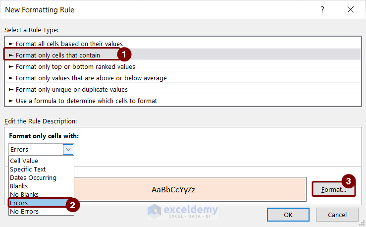
- In the New Formatting Rule window, select Format only cells that contain.
- Choose Blanks from the dropdown to highlight blank cells.
- Optionally, you can select other options like Cell Value, Specific Text, Dates Occurring, No errors, or No Blanks.
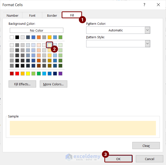
- Set a fill color and click OK in both windows.
- To highlight Errors, select the Errors option to highlight the cells with errors.
- Choose light yellow fill color to differentiate between the blanks and errors.
- Now, you will have the dataset highlighting the Blanks and Errors.
Read More: Conditional Formatting If Cell Is Not Blank
Highlighting Odd or Even Rows with Conditional Formatting
- Go to the New Rule option in Conditional Formatting.
- Select the Use a Formula to determine which cells to format option as the rule type.
- Enter the following formula into the box:
=ISODD(ROW())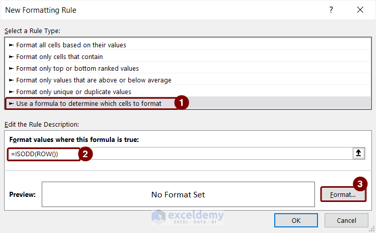
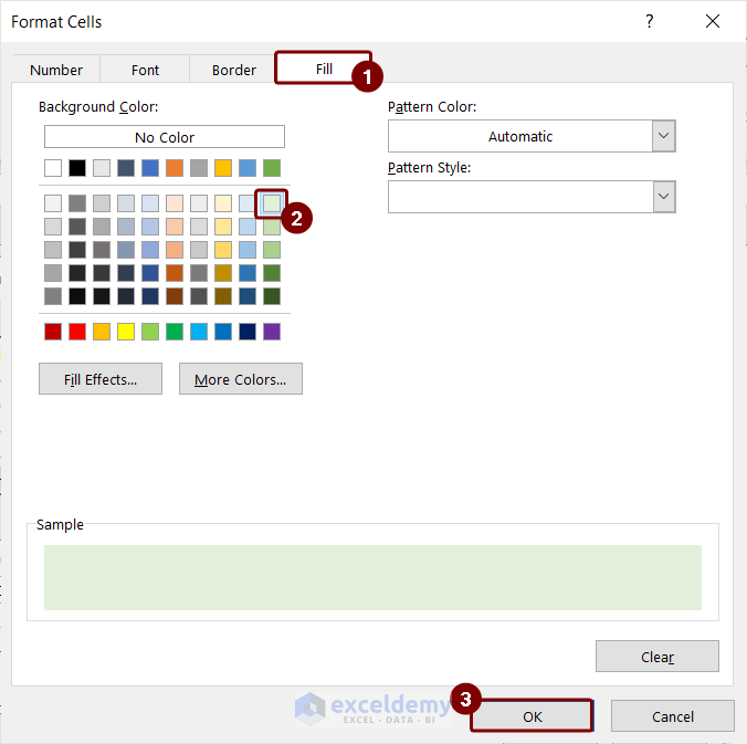
- Click on the Format button and select a fill color to highlight.
- Press OK.
- Recheck the formatting rule and press OK.
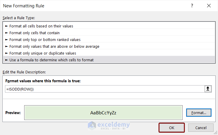
- You get the dataset as shown in the below screenshot.
=ISEVEN(ROW())Highlight Every nth Row
- Go to the New Rule option in Conditional Formatting.
- Select the “se a Formula to determine which cells to format option as the rule type.
- Enter the following formula into the box to format every 3rd row (you can adjust the number as needed):
=MOD(ROW(),3)=0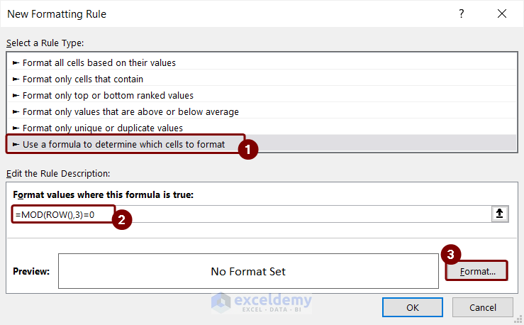
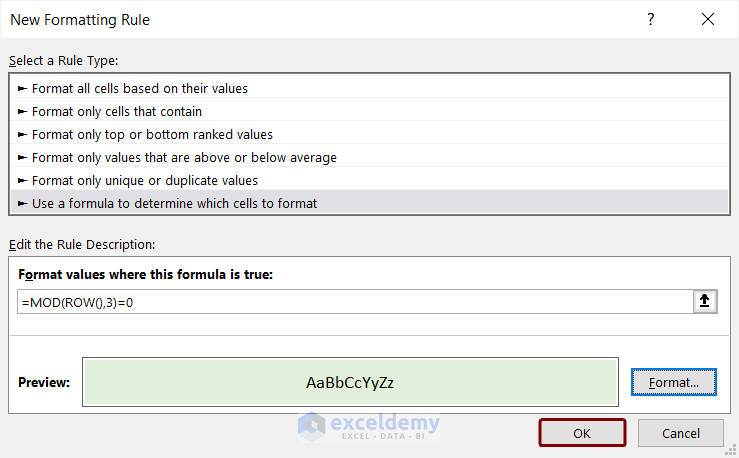
- Click on the Format button and select a fill color to highlight.
- Press OK.
- Press OK after checking the formatting rule.
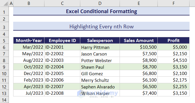
- As a result, you will see that the 6th, 9th, and 12th-row cells of the dataset have become filled with color.
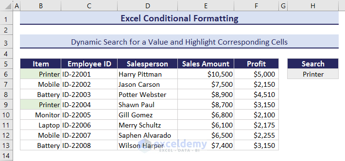
Dynamic Search and Highlight Corresponding Cells
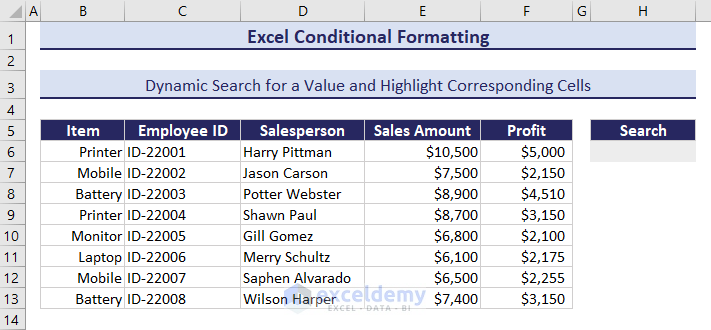
- Select the range B6:B13.
- Go to the New Rule option in Conditional Formatting.
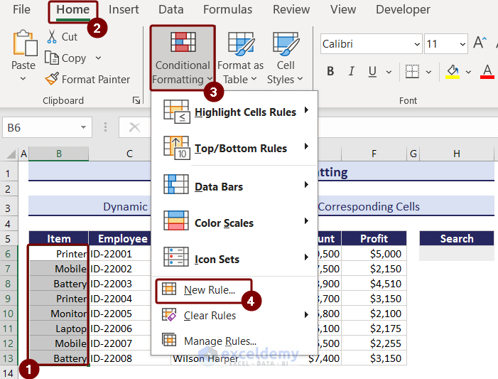
- Here, select the Use a Formula to determine which cells to format option as the rule type.
- Enter the following formula into the box:
=AND($H$6<>"",$H$6=B6)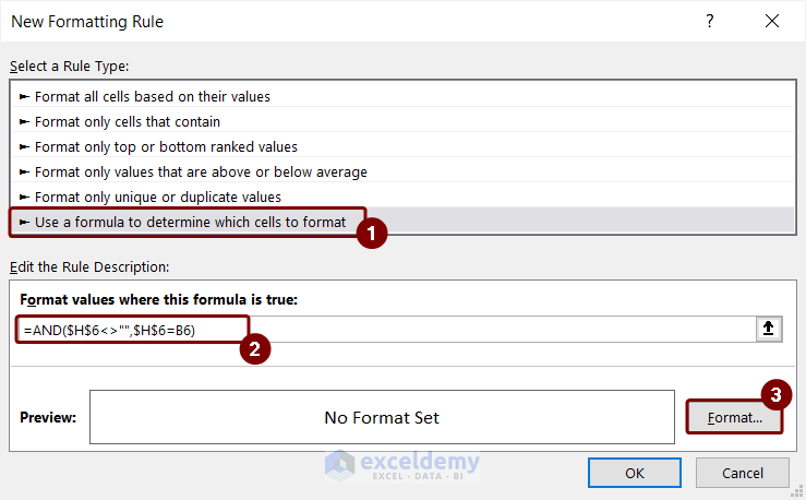
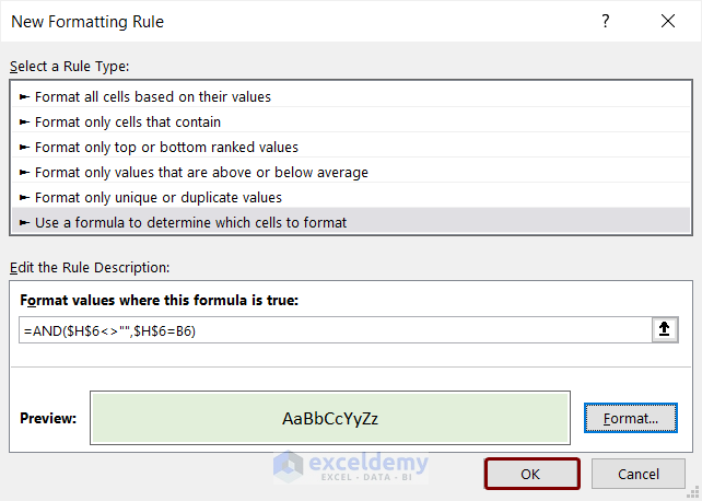
- Click on the Format button and select a fill color.
- Press OK.
- Confirm the formatting and press OK.
- When you input a value into cell F5, the corresponding cell in the dataset will be highlighted.
- If we type Printer, then the cells with this input in range B6:B13 get highlighted.
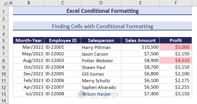
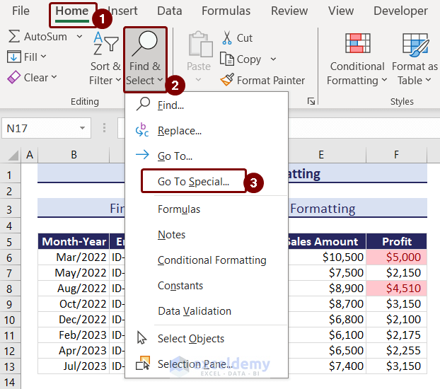
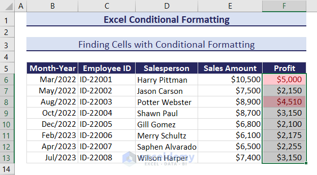
Finding Cells with Conditional Formatting
- Open your Excel dataset.
- Click on the Home tab in the Excel ribbon.
- Under the Editing group, choose Find & Select and then select Go To Special.
- In the Go To Special dialog box, select Conditional Formats and click OK.
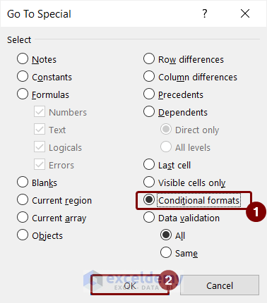
- The cells with conditional formatting will be highlighted.
Removing Conditional Formatting
To remove conditional formatting from a specific range (e.g., F6:F13):
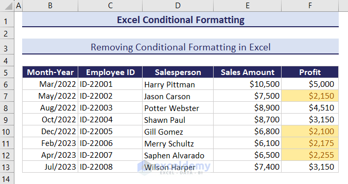
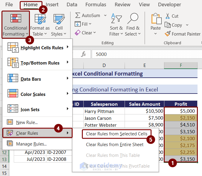
- Select the range of cells (F6:F13).
- Go to the Home tab.
- Under Conditional Formatting, choose Clear Rules and select either Clear Rules from Selected Cells or Clear Rules from Entire Sheet.
- To delete specific formatting rules:
- Select the cells with conditional formatting.
- Click on Manage Rules in the Conditional Formatting menu.
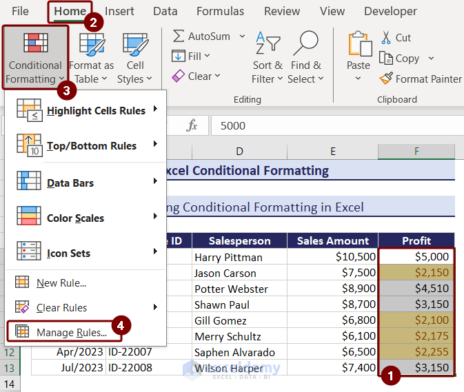
- Choose the rule you want to delete (e.g., Cell Value < 3000).
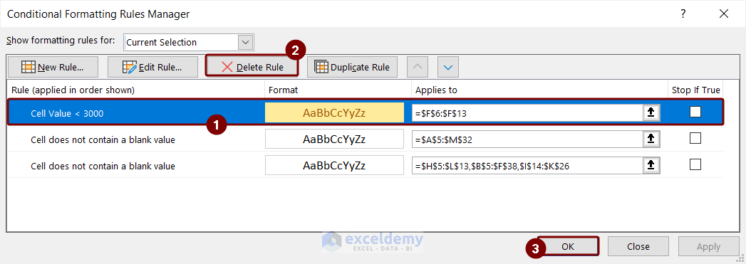
Click the image to get a better view
- Click Delete Rule and confirm.
Read More: How to Remove Conditional Formatting but Keep the Format
Download Practice Workbook
You can download the practice workbook from here:
Conditional Formatting in Excel: Knowledge Hub
- Apply Different Types of Conditional Formatting
- Find External Links in Conditional Formatting
- Apply Conditional Formatting for Blank Cells
- Apply Conditional Formatting on Multiple Columns
- Compare Two Columns Using Conditional Formatting
- Remove Conditional Formatting
- Remove Conditional Formatting but Keep the Format
- Apply Conditional Formatting to the Selected Cells
- Make Yes Green and No Red
- Create a Rating Scale
- Use Conditional Formatting on Text Box
- Apply Borders in Excel with Conditional Formatting
- Apply Alignment in Excel Conditional Formatting
- Conditional Formatting with Formula
- Applying Conditional Formatting for Multiple Conditions
- Excel Conditional Formatting Based on Date
- Apply Conditional Formatting to Multiple Rows
- Data Bars in Excel
- Use Conditional Formatting Icon Sets
<< Go Back to Learn Excel
Get FREE Advanced Excel Exercises with Solutions!

Excel has huuuuuge to know, to fabricate data.
This is the tool for that.
Aziz Bro, thanks for your comments. Excel has extended its power more in recent times making Excel to work with Microsoft’s Power BI tools. I shall focus on them within very short time. Keep in touch. Thanks again.
It would be good to have a small section about how to format conditionally using, for instance, values in the same row or in the same column. The formatting would then be applied to a rectangular range and that would be done based on a formatting formula that one types in the formatting dialog box. There are some rules about how to do it for ranges based on just one cell in the entire range. It’s all about using relative and absolute cell references. This is exactly what’s missing from the above text but, of course, does NOT make the text in any way wrong or unuseble.
Hello Mr. Kawsar, Thank you for this valuable information.
I am trying to write an if function or use conditional formatting that can do the following task:
Search for all cells in the worksheet that contains a certain “text” and Highlight them, if a formula is true.
Example: If (A2=”US” then search for all cells in the worksheet that contains “United States” and highlight them Red).
I hope this can be done, looking forward to hearing from you. Thank you
Dear Jamil,
Using conditional formatting you can search for a specific text and color them according to your choice. Follow the instructions below.
Suppose we have a dataset of some countries’ names in cells (B3:E9). Now we are going to color a specific text (United States) from the list.
First, select all the cells and click the “Text that contains” option from the “Conditional Formatting” feature.
Second, put your desired text and choose a color of your choice. Gently, press OK.
Finally, we have successfully highlighted a certain text from the list.
Hope you got the solution you are looking for. If you still having problems then check the link below. Thanks!
Highlight Cells Based on Text
Hi,
Thanks for the information. In my situation, after I have applied a manual format and two other conditional format rules on fill color, my cells display the right color based on that conditional format rules take precedence over manual format. However, if I right click the cell and open the “Format Cells..” dialog, the fill color recorded in the system for that cell is still the manual formatted color no matter what the conditional format rule is. Since I will need to sum certain cells based on their fill color, to have the right color not just displayed, but also recorded in the system, is very important. Hope I can get an answer. Appreciate your help!
Dear RUBY,
Here is the solution you are looking for.
Suppose you have a dataset with conditional formatting applied in the list.
First, select all the cells (C2:C11) from the column and click the “Filter” option from the “Data” ribbon.
Now press the “Filter icon and choose “Filter by Color”. Hence choose your cell color.
Thereafter, you will get to see only the cells with the selected colors. Let’s calculate the total sum now. To do so, choose a cell (C13) and writhe the following formula down-
=SUBTOTAL(109,C3:C11)
Finally, you will get the sum value for the colored cells only.
If you are still facing problems then you can read this article – How to Sum Colored Cells in Excel
Thanks!
@ Ruby
Thanks for sharing very nice information