In this article, we will describe 3 easy ways to find and highlight duplicates in Excel, and some other useful methods for dealing with duplicate rows and cell values.
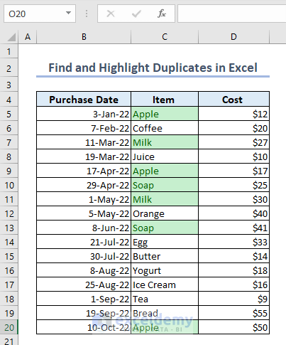
Here is an overview:
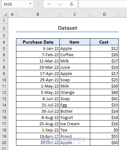
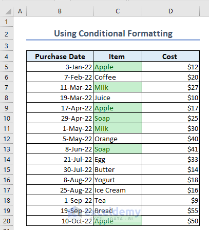
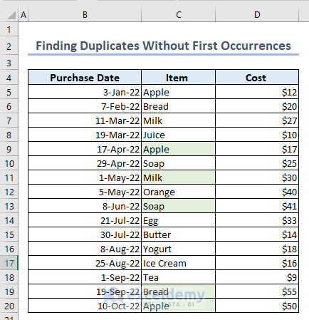
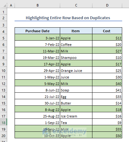
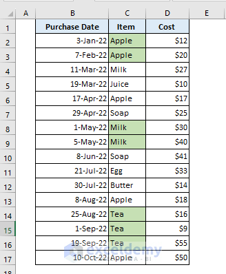
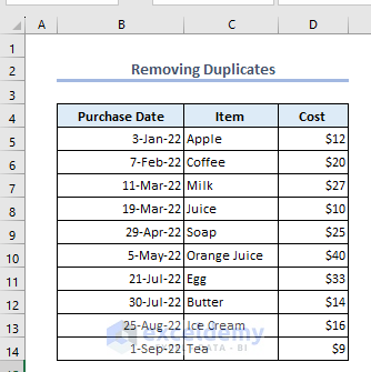
Suppose we have the following dataset containing columns for the Purchase Date, Item, and Cost of some purchases. The Item column contains numerous duplicates. Let’s find and highlight them.
Example 1 – Finding and Highlighting Duplicates in a Single Column
1.1 – Using Conditional Formatting
Here, we will highlight duplicates including their first occurrences.
Steps:
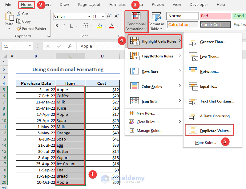
- Select the range of cells in which to find duplicates. Here, we select the entire Item column.
- Go to the Home tab.
- From the Conditional Formatting group, select Highlight Cells Rule.
- Select Duplicate Values.
A Duplicate Values dialog box opens.
- Select Duplicate.
- Select a color type, such as Green Fill with Dark Green Text.
- Click OK.
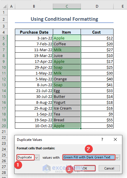
The duplicates are highlighted in light green.
Read More: Find Duplicates in Two Columns in Excel
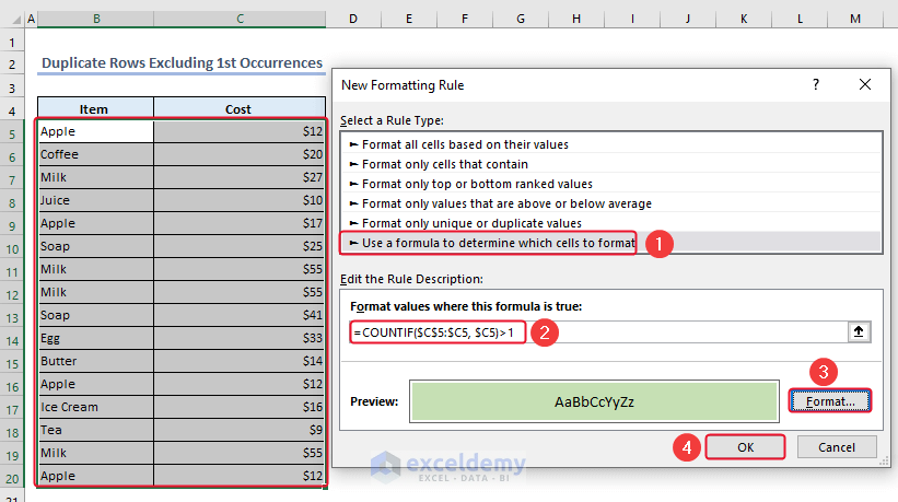
1.2 – Find and Highlight Duplicates Excluding the First Occurrences
Here, we will find and highlight duplicate values but not the first occurrences.
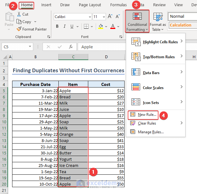
- Select the entire Item column.
- Go to the Home tab.
- From the Conditional Formatting group, select New Rule.
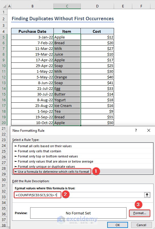
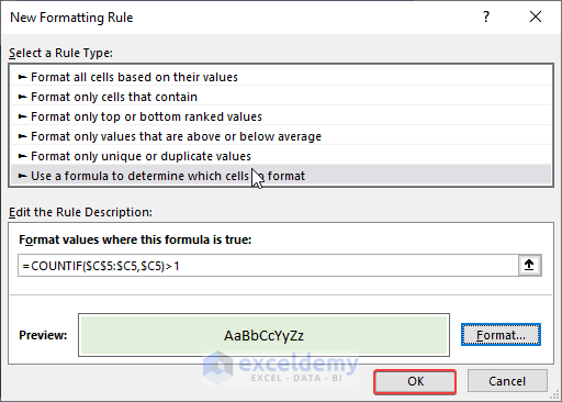
A New Formatting Rule dialog box will appear.
- Select Use a formula to determine which cells to format.
- Enter the following formula in the formula box:
=COUNTIF($C$5:$C5,$C5)>1- Click on Format.
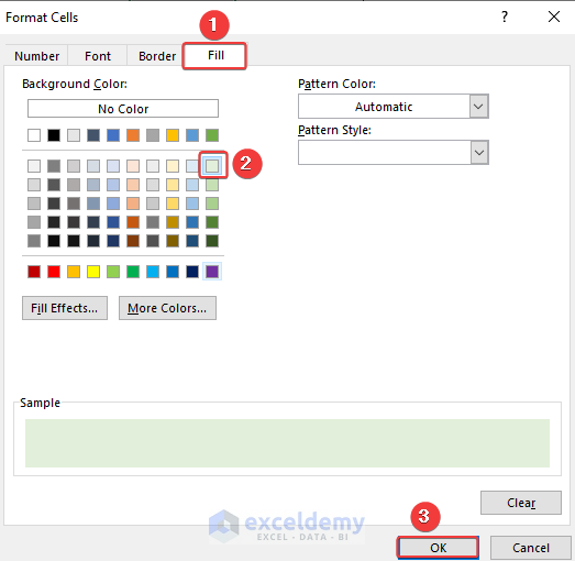
A Format Cells dialog box will appear.
- Go to the Fill tab.
- Select a Color and click OK.
In the New Formatting Rule dialog box, the Preview of the Color is shown.
- Click OK.
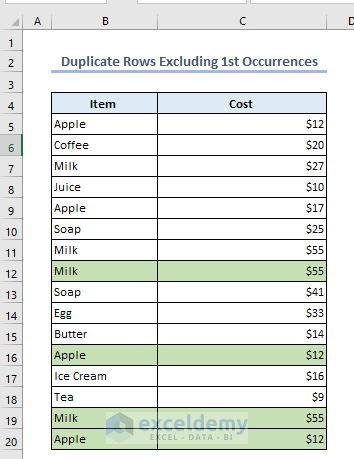
The duplicates are highlighted, but the first occurrences aren’t.
Read More: Excel Formula to Find Duplicates in One Column
Example 2 – Finding and Highlighting Duplicates in Multiple Columns
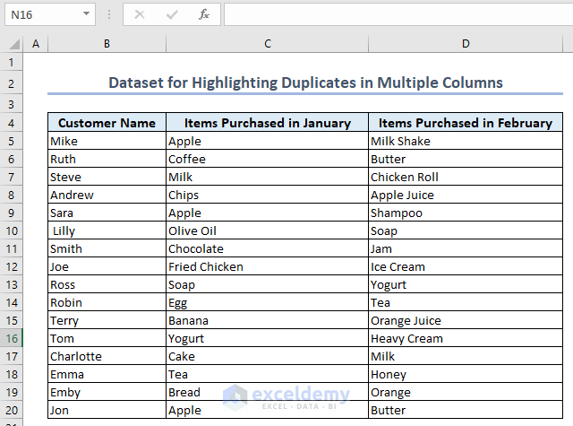
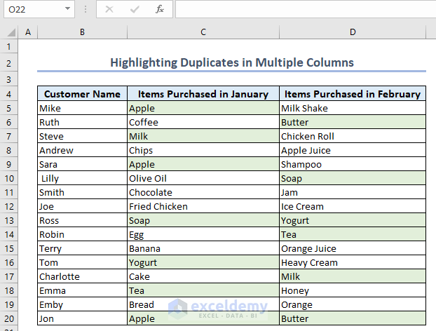
In the following dataset, we have columns for Customer Name, Items Purchased in January, and Items Purchased in February. Both the Items Purchased in January and Items Purchased in February columns have several duplicates.
Using this dataset, we will find and highlight duplicates in multiple columns.
2.1 – Highlighting Duplicates Including First Occurrences
We will use the COUNTIF function here.
Steps:
- Select the entire Items Purchased in January and Items Purchased in February columns excluding the column headings.
- Follow the Steps described in Example 1.2 to open the New Formatting Rule dialog box and the formula box.
- Enter the following formula in the formula box:
=COUNTIF($C$5:$D$20, C5)>1- Click on Format and format the cells as desired.
- Click OK.
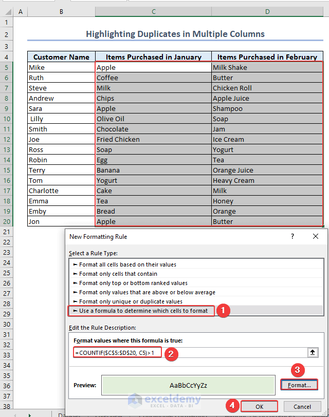
We have found and highlighted duplicate values in multiple columns, including the first occurrences of those values.
Read More: How to Find Duplicates in Excel Workbook
2.2 – Highlighting Duplicates Without the First Occurrences
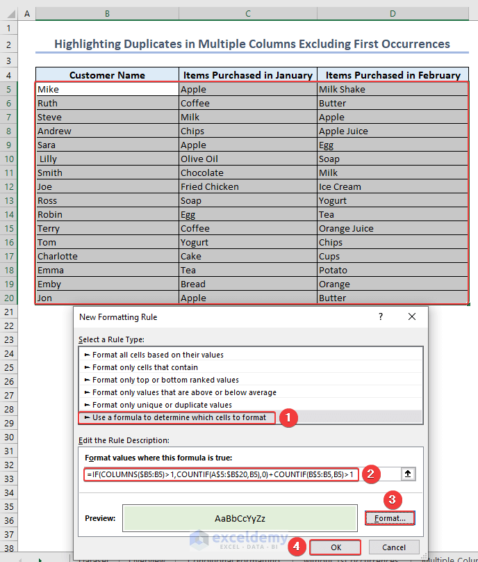
Now we will highlight duplicate values in multiple columns excluding the first occurrences, using the combination of the IF and COUNTIF functions.
Steps:
- Select the entire Items Purchased in January and Items Purchased in February columns, excluding the column headings.
- Follow the Steps described in Example 1.2 to open the New Formatting Rule dialog box and the formula box.
- Enter the following formula in the formula box:
=IF(COLUMNS($B5:B5)>1,COUNTIF(A$5:$B$20,B5),0)+COUNTIF(B$5:B5,B5)>1- Click on Format and format the cells as desired, then click OK.
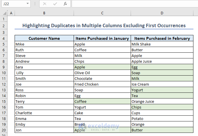
Duplicate values are highlighted in multiple columns, excluding the first occurrences of those values.
Read More: How to Find Similar Text in Two Columns in Excel
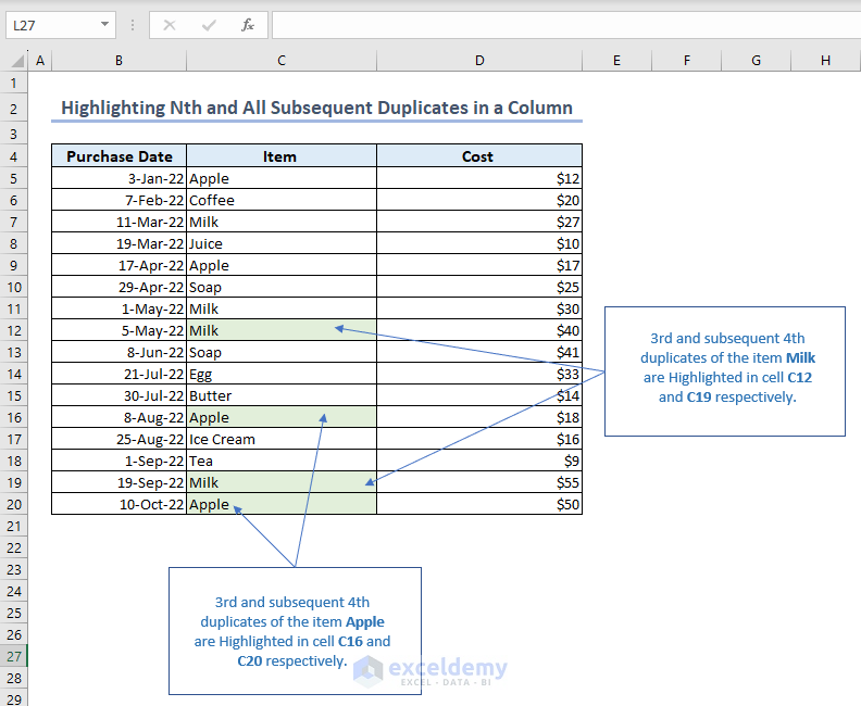
Example 3 – Finding and Highlighting the Nth Subsequent Duplicate
Now we will find the nth subsequent duplicate in a dataset, for example the 3rd, 4th, or any subsequent duplicate. In particular, we’ll find the 3rd and all subsequent duplicates, and then the 3rd duplicate only.
3.1 – Finding and Highlighting the Third and All Subsequent Duplicates
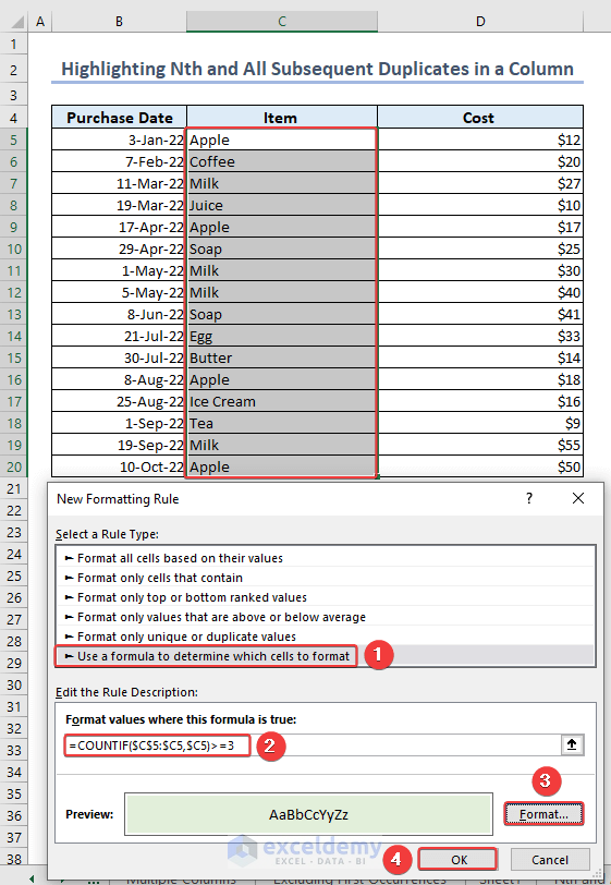
Let’s find and highlight the 3rd and all subsequent duplicates in the column Item.
- Select the column Item.
- Follow the Steps described in Example 1.2 to open the New Formatting Rule dialog box.
- Enter the following formula in the formula box:
=COUNTIF($C$5:$C5,$C5)>=3- Click on Format and format the cells as desired.
- Click OK.
Note: To find the 2nd or 4th duplicate, just input 2 or 4 in the above formula instead of 3.
Thus, the formula will be:
=COUNTIF($C$5:$C5,$C5)>=2 for the 2nd and all subsequent duplicates.
=COUNTIF($C$5:$C5,$C5)>=4 for the 4th and all subsequent duplicates.
The result is as in the following image.
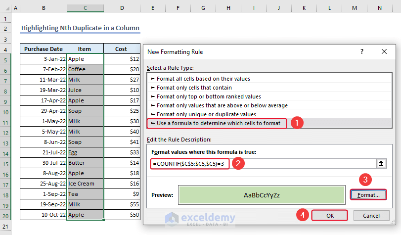
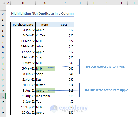
3.2 – Finding and Highlighting the Third Duplicates Only
Here, we will find only the 3rd duplicates of Items.
- Select the column Item.
- Follow the Steps described in Example 1.2 to open the New Formatting Rule dialog box.
- Enter the following formula in the formula box:
=COUNTIF($C$5:$C5,$C5)=3- Click on Format and format the cells as desired.
- Click OK.
Note: To find the 2nd or 4th duplicate, just input 2 or 4 in the above formula instead of 3.
Thus, the formula will be:
=COUNTIF($C$5:$C5,$C5)=2 for the 2nd duplicate.
=COUNTIF($C$5:$C5,$C5)=4 for the 4th duplicate.
The result is as in the image below.
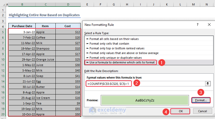
Highlighting Entire Rows When Only One Column Contains Duplicates
In our dataset, the Purchase Date and Cost columns contain no duplicates, but the Item column does. Let’s highlight the entire row based on duplicate Item values.
Including First Occurrences:
Steps:
- Select the entire dataset excluding the column headings.
- Follow the Steps described in Example 1.2 to open the New Formatting Rule dialog box.
- Enter the following formula in the formula box:
=COUNTIF($C$5:$C$20, $C5)>1- Click on Format and format the cells as desired.
- Click OK.
The entire rows containing duplicate items are highlighted.
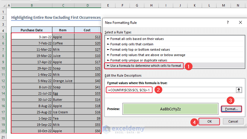
Excluding First Occurrences:
- Select the entire dataset.
- Follow the Steps described in Example 1.2 to open the New Formatting Rule dialog box.
- Enter the following formula in the formula box:
=COUNTIF($C$5:$C5, $C5)>1- Click on Format and format the cells as desired.
- Click OK.
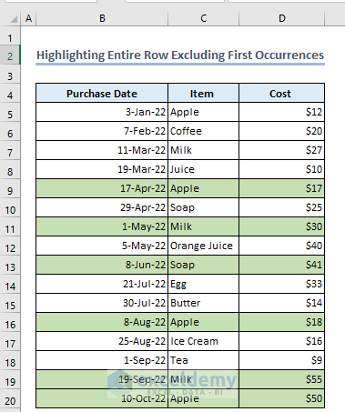
The entire rows containing duplicate values are highlighted, excluding those containing the first occurrences.
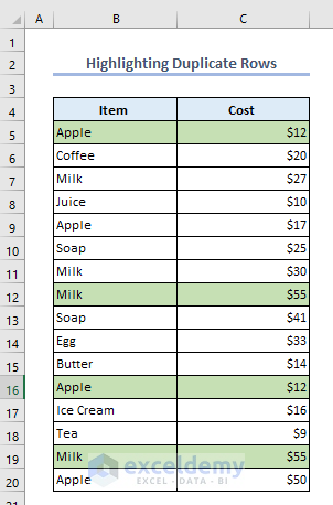
Highlight the Duplicate Rows Only
The previous examples dealt with duplicate cell values. Now we will highlight duplicate rows.
Including First Occurrences:
- Select the whole dataset.
- Follow the Steps described in Example 1.2 to open the New Formatting Rule dialog box.
- Enter the following formula in the formula box:
=COUNTIFS($B$5:$B$20, $B5, $C$5:$C$20, $C5)>1- Click on Format and format the cells as desired.
- Click OK.
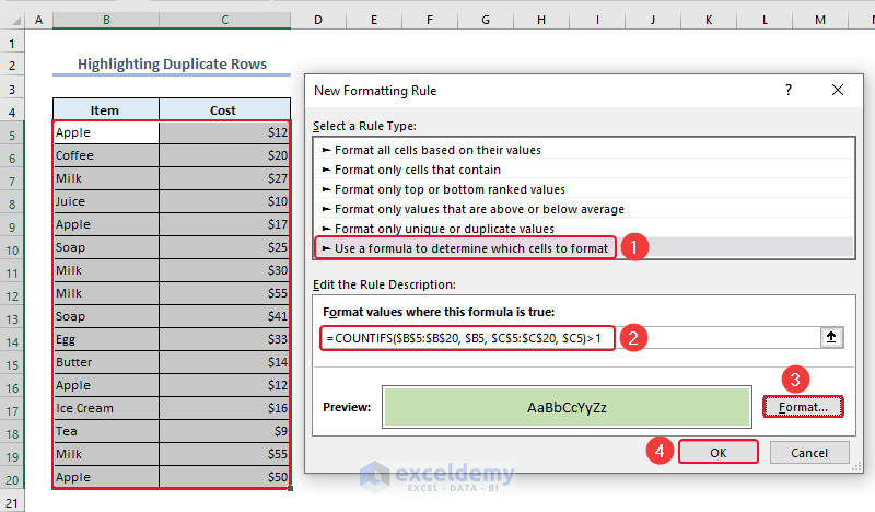
The duplicate rows are highlighted.
Excluding First Occurrences:
- Select the whole dataset.
- Follow the Steps described in Example 1.2 to open the New Formatting Rule dialog box.
- Enter the following formula in the formula box:
=COUNTIF($C$5:$C5, $C5)>1- Click on Format and format the cells as desired.
- Click OK.
The duplicate rows excluding the first occurrences are highlighted.
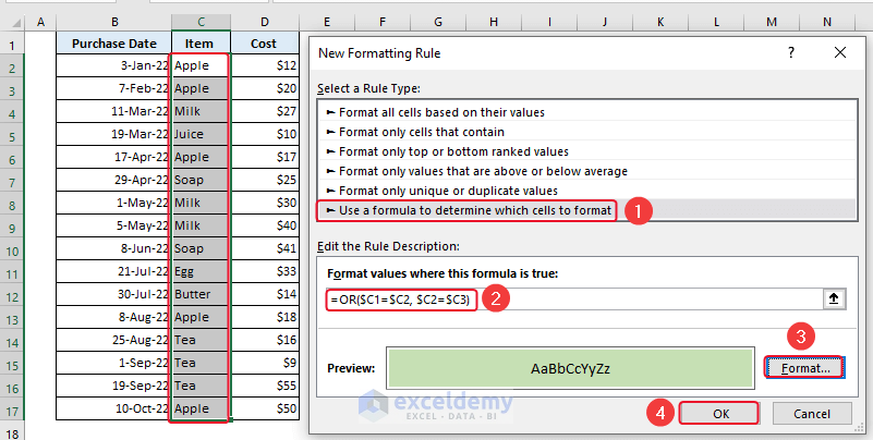
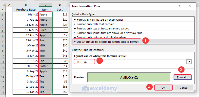
Finding and Highlighting Consecutive Duplicate Cells
Now, we will find and highlight the consecutive duplicate cells in the Item column.
Including First Occurrences:
- Select the Item column.
- Follow the Steps described in Example 1.2 to open the New Formatting Rule dialog box.
- Enter the following formula in the formula box:
=OR($C1=$C2, $C2=$C3)- Click on Format and format the cells as desired.
- Click OK.
The cells containing consecutive duplicates are highlighted.
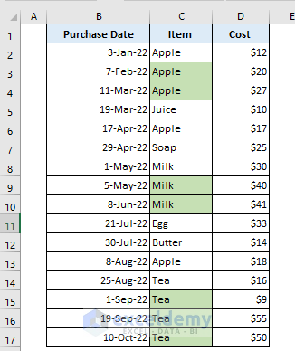
Excluding First Occurrences:
- Select the Item column.
- Follow the Steps described in Example 1.2 to open the New Formatting Rule dialog box.
- Enter the following formula in the formula box:
=$C1=$C2- Click on Format and format the cells as desired.
- Click OK.
The output is as in the following image.
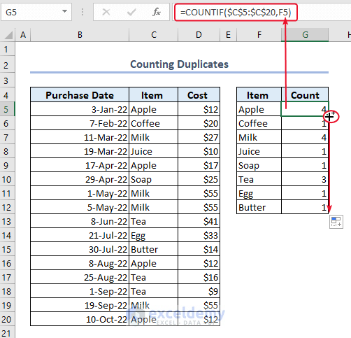
How to Count Duplicates in Excel
Steps:
- Enter the following formula in cell G5:
=COUNTIF($C$5:$C$20,F5)- Press ENTER to return the result.
- Drag down the formula with the Fill Handle tool.
The count of every item including duplicates is displayed in cells G5:G12.
How to Remove Duplicates in Excel
In the following dataset, we have duplicates in the Item column. Let’s remove them.
Steps:
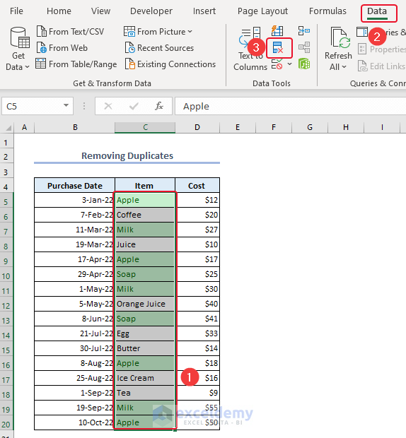
- Select the entire Item column.
- Go to the Data tab.
- From the Data Tools group, click on Remove Duplicates.
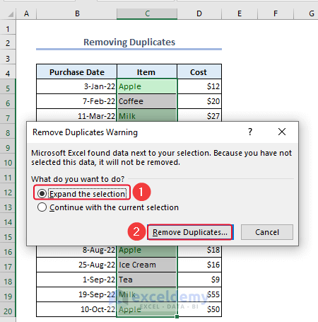
A Remove Duplicates Warning dialog box will appear.
- Click Expand the Selection >> click Remove Duplicates.
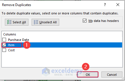
- In the Remove Duplicates dialog box, mark Item and click OK.
We marked Item only since only the Item column contains duplicates.
- Click OK in the confirmation dialog box.
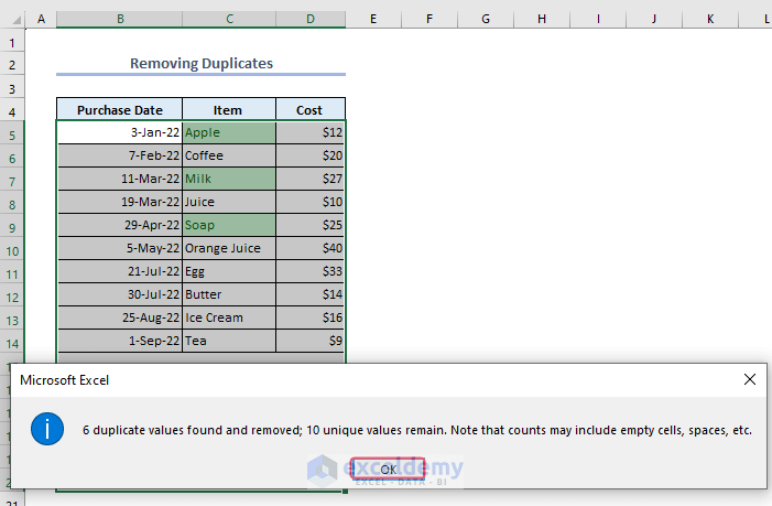
We have removed all the duplicates.
Read More: How to Find Duplicates without Deleting in Excel
Things to Remember
- Select the correct range of cells before applying Conditional Formatting.
- If the dataset has merged cells, unmerge them before applying methods to find duplicates, or the methods may not work as intended.
- Select a color in the Format option of the New Formatting. Otherwise, Excel will identify the duplicates but we won’t be able to see them.
Download Practice Workbook
Related Articles
- How to Find Duplicate Values Using VLOOKUP in Excel
- How to Find Duplicates in Two Different Excel Workbooks
<< Go Back to Find Duplicates in Excel | Learn Excel
Get FREE Advanced Excel Exercises with Solutions!
