Excel Formula to Find Duplicates in One Column (8 Easy Ways)

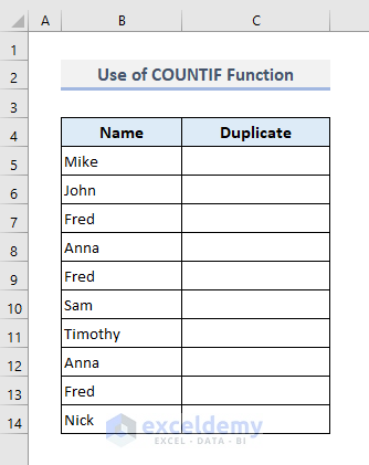
Method 1 – Using the COUNTIF Function to Find Duplicates in One Column Along with the First Occurrence

We have a list of names in column B. The formula to find duplicates will return TRUE for duplicate names and FALSE for unique ones in column C.

• Insert the following formula in the first result cell (C5), then press Enter and use AutoFill to get the results throughout the column.

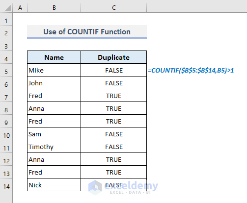
The COUNTIF function returns the number of counts for each name (second argument). The logical operator checks for counts that are greater than 1.

Read More: Find Duplicates in Two Columns in Excel

Method 2 – Creating an Excel Formula with IF and COUNTIF Functions to Find Duplicates in One Column

Under the Output header, the formula will return Duplicate for the duplicate names present in Column B.

• Insert the following formula in the first result cell (C5), then press Enter and use AutoFill to get the results throughout the column.

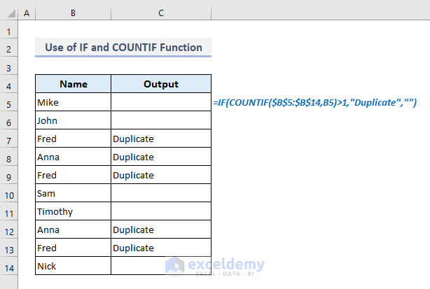
The IF function wraps the formula from Method 1 to return the specified text Duplicate or a blank value.

Read More: How to Find Similar Text in Two Columns in Excel

Method 3 – Finding Duplicates in One Column Without the First Occurrence in Excel

The formula will display Duplicate only if a value has already been repeated previously (i.e., the first occurrence will get a blank result).

• Insert the following formula in the first result cell (C5), then press Enter and use AutoFill to get the results throughout the column.

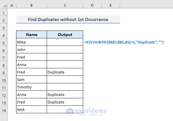
For the first output in Cell C5, we’ve defined the cell range with $B$5:$B5 so the second row reference moves with the formula. For each subsequent output, the number of cells in the defined range for the COUNTIF function increases by 1. This ensures that the first value will only be counted once.

Method 4 – Using Excel Formula to Find Case-Sensitive Duplicates in a Single Column

• Insert the following formula in the first result cell (C5), then press Enter and use AutoFill to get the results throughout the column.

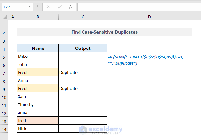
How Does the Formula Work?

• The EXACT function here looks for the case-sensitive and exact matches for the first text in the Name column and thereby returns the following output:

{TRUE;FALSE;FALSE;FALSE;FALSE;FALSE;FALSE;FALSE;FALSE;FALSE}

• With the use of double-unary (–), the return values TRUE and FALSE convert into numbers 1 and 0. So, the return values here will be:

{1;0;0;0;0;0;0;0;0;0}

• The SUM function then sums up all the numeric values found in the preceding step.
• =SUM((–EXACT($B$5:$B$14, B5)))<=1: This part of the formula checks if the sum or the return value found in the last step is equal to or less than 1.
• The IF function looks for the sum less than or equal to 1 and returns a blank cell, and if not found then it returns the defined text Duplicate.

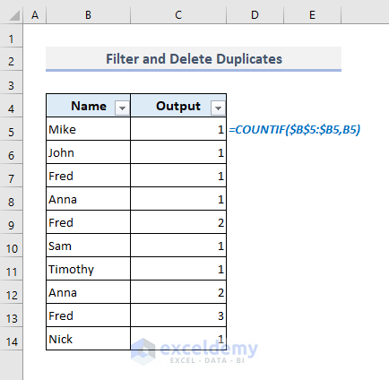
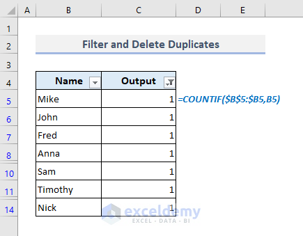
Method 5 – Finding How Many Times a Value Has Been Repeated in a Column

• Insert the following formula in the first result cell (C5), then press Enter and use AutoFill to get the results throughout the column.

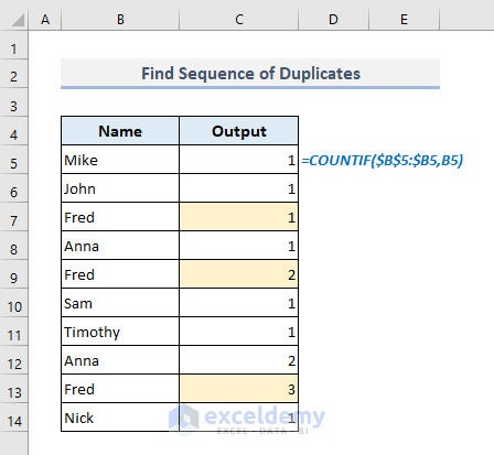
This formula is similar to the one used to check duplicates without the first occurrence, with the second reference moving with the formula. The COUNTIF function naturally returns a number, so we don’t need any more checks.

Method 6 – Filtering and Deleting Duplicates in One Column in Excel

We’ve used Method 5 to get the serial number of each value’s occurrence.

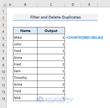
Steps:

• Select the entire table, including its headers.
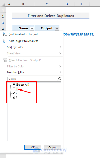
• Under the Home tab, select the option Filter from the Sort & Filter drop-down in the Editing group of commands.

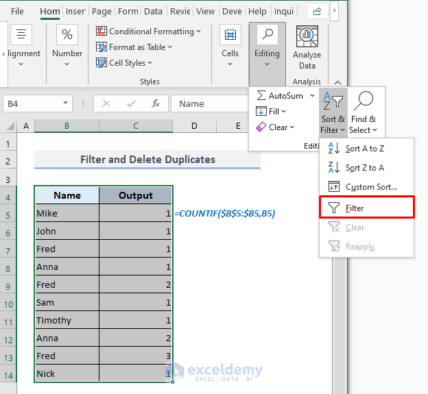
• This activates the Filter buttons for the headers.

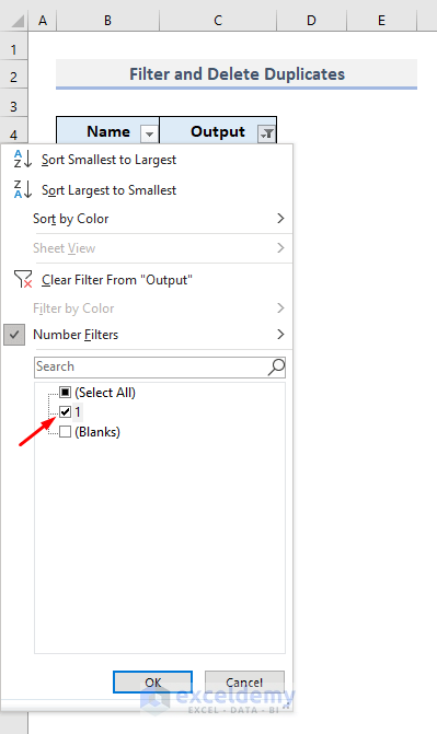
• Click on the Output drop-down and unmark 1.
• Click OK.

• You’ll get a list of duplicated values.

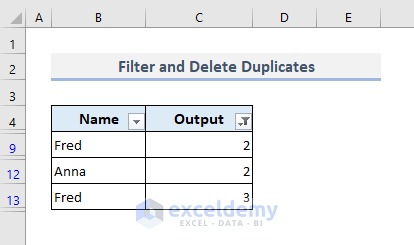
• Select these cells and delete them.

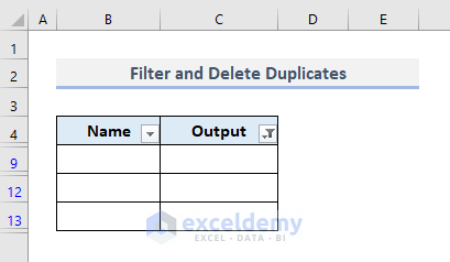
• Open the Output filter again.
• Mark the option 1 only.
• Click on OK.

• You’ll get all the unique text data or names only. The cells with blank values have been hidden with the filter. You can remove those rows afterward.

Read More: How to Find Duplicates without Deleting in Excel

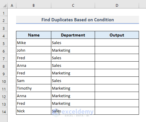
Method 7 – Creating an Excel Formula to Find Duplicates in One Column Based on a Condition

We have an additional column that represents the departments for all employees in an organization. We’ll check if we have duplicated combinations of name and department.

• Insert the following formula in the first result cell (D5), then press Enter and use AutoFill to get the results throughout the column.

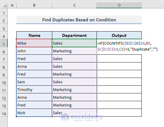
• Here’s the result.

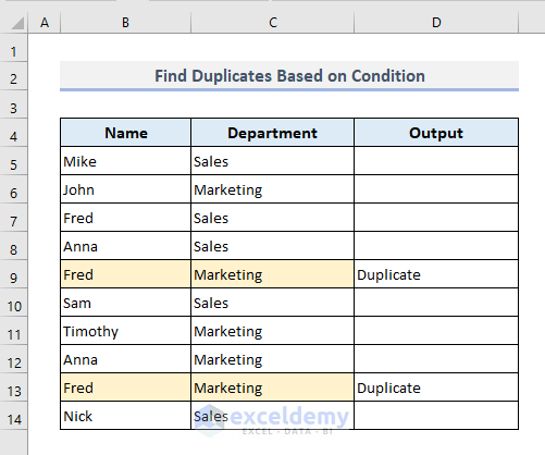
The COUNTIFS function implicitly uses the AND argument between all conditions and their ranges.

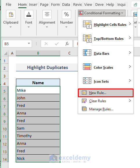
Method 8 – Finding and Highlighting Duplicates with Conditional Formatting

• Select all the names under the Name header in Column B.
• Under the Home ribbon, choose the option New Rule from the Conditional Formatting drop-down.
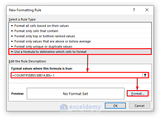
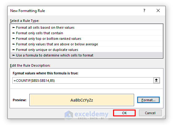
• A dialog box named New Formatting Rule will appear.

• Select the Rule Type as Use a formula to determine which cells to format.
• In the Rule Description box, insert the following formula:

• Press Format.

• In the Format Cells window, switch to the Fill tab and select a background color for the duplicate cells.
• Press OK.

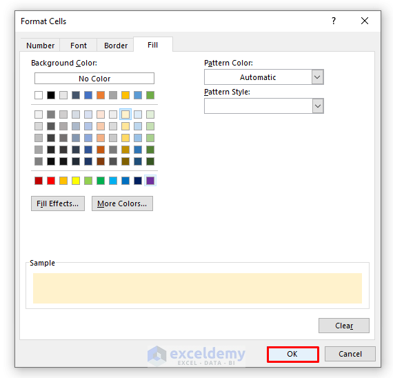
• You’ll find a preview of the format of the cell as shown in the picture below. Click OK.

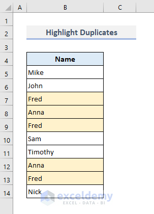
• The formula highlights all duplicates including their first occurrences. You can use a different formula to highlight only the occurrences after the first (see Method 3).

Read More: How to Find Duplicate Values Using VLOOKUP in Excel

Download the Practice Workbook

Related Articles

• How to Find Duplicates in Excel Workbook
• How to Find Duplicates in Two Different Excel Workbooks

<< Go Back to Find Duplicates in Excel Column | Find Duplicates in Excel | Learn Excel