Method 1 – Use VLOOKUP to Find Duplicate Values in Two Columns
Make two columns that contain different product names. Look for the Product Name-1 column names in the Product Name-2 column. This is the formula to find duplicates that we are going to use:
=VLOOKUP(List-1, List-2,True,False)In this formula, the List-1 names will be searched in List-2. If there exists any duplicate name, the formula will return the name from List-1.
Steps:
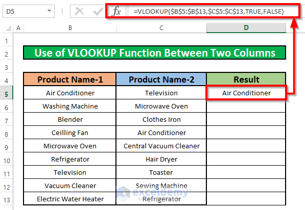
- Select cell D5, and write down the VLOOKUP function in that cell.
=VLOOKUP($B$5:$B$13,$C$5:$C$13,TRUE,FALSE)- Press Enter on your keyboard. Get the duplicate value which is the return value of the VLOOKUP function.
- The Air Conditioner is found because the VLOOKUP function searches this name from Product Name-1 to Product Name-2. The result from Product Name-1 will be output when the name is found.
- Drag down the formulated cell D5 downwards to complete the result for the two columns.
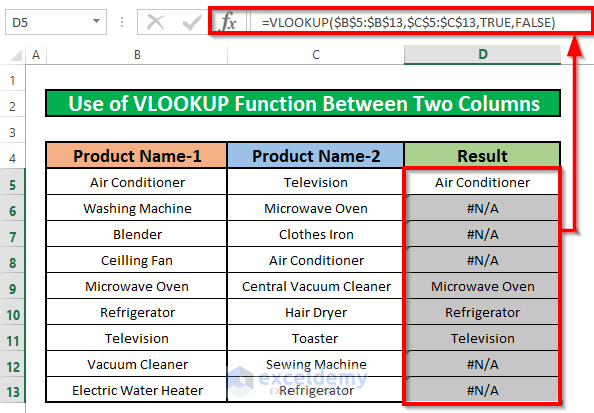
- The #N/A results are found because, in those particular cells, the names from column B are not found in column C.
- In the Result column, 4 duplicate values (Air Conditioner, Microwave Oven, Refrigerator, and Television). #N/A values are representing the unique values of column Product Name-1.
Method 2 – Apply VLOOKUP to Find Duplicate Values in Two Excel Worksheets
Steps:
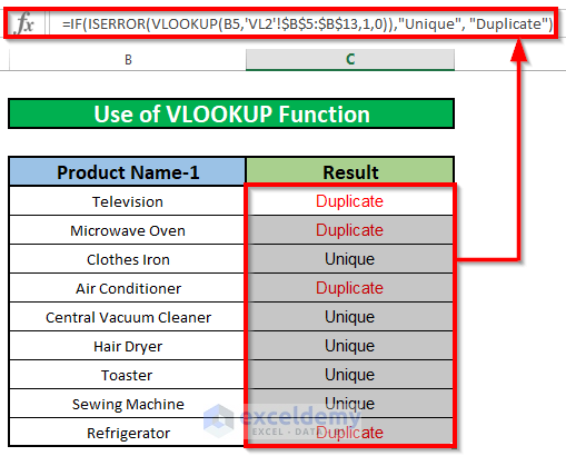
- In C5 of VL3, type the below formula.
=IF(ISERROR(VLOOKUP(B5,'VL2'!$B$5:$B$13,1,0)),"Unique", "Duplicate")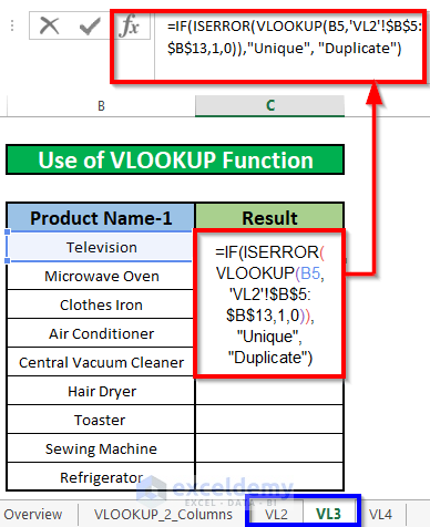
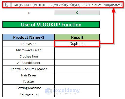
- Press ENTER on your keyboard. See the result Duplicate because the name Television exists in VL2.
- Drag this formulated cell C5 to carry out the result for the rest of the cells in column C.
- For a proper view, look at the GIF.
Method 3- Insert VLOOKUP to Find Duplicates in Two Workbooks of Excel
- Created a new workbook titled VL and in the workbook create a new worksheet titled Sheet1. In Sheet1 create a product list just like before.
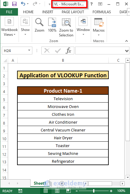
- In the main workbook, which we were working on (in our last example), create another worksheet titled VL4 and again create a list of products.
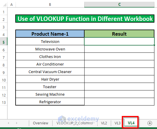
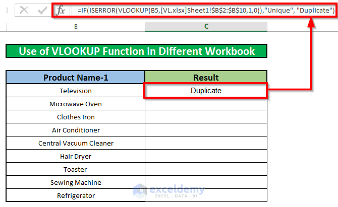
- In cell C5 of VL4, write the following formula and press ENTER.
=IF(ISERROR(VLOOKUP(B5,[VL.xlsx]Sheet1!$B$2:$B$10,1,0)),"Unique", "Duplicate")- See the results duplicate as Television exists in VL4.
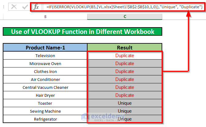
- Drag the formulated cell C5 to see the result for the remaining cells in column C.
- Find out the duplicates between the two workbooks.
Bottom Line
➜ While a value can not be found in the referenced cell, the #N/A! The error happens in Excel.
➜ #DIV/0! error happens when a value is divided by zero(0) or the cell reference is blank.
Download Practice Workbook
Download these two practice workbooks to exercise while you are reading this article.
Related Articles
- How to Find Duplicates without Deleting in Excel
- Find and Highlight Duplicates in Excel
- Find Duplicates in Two Columns in Excel
- How to Find Similar Text in Two Columns in Excel
<< Go Back to Find Duplicates in Excel | Learn Excel
Get FREE Advanced Excel Exercises with Solutions!

This is brilliant! May I share the link to this article with another online class that I am taking?
Hi Stanley,
Thanks for the comments. Glad to hear that it is helpful. Yes. You can share it with an online class with an attribution to our blog.
Best regards
It would be most helpful if the “Download” file was in Excel. Thank you
When we have more than one files for an article, we make a compressed file.
Hope you understand. Other articles that have just the Excel file to share, the download options are in Excel File.
Best regards
Kawser Ahmed
Is there a way to have this kind of formula that shows count of duplicates in a single column? I am interested to know if there is a “formula-way” to count how many unique cells and how many duplicates in a single column without referencing other column.
Thanks for reaching out. Kindly mail me your Excel file and queries at [email protected]
I’ll be happy to help.
very helpful post for excel beginner and expert candidate
Thanks, glad we could help you.