How to Find Similar Text in Two Columns in Excel

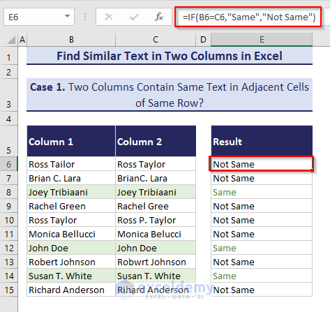
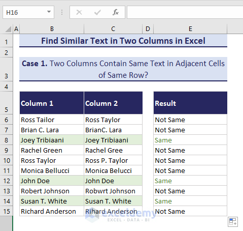
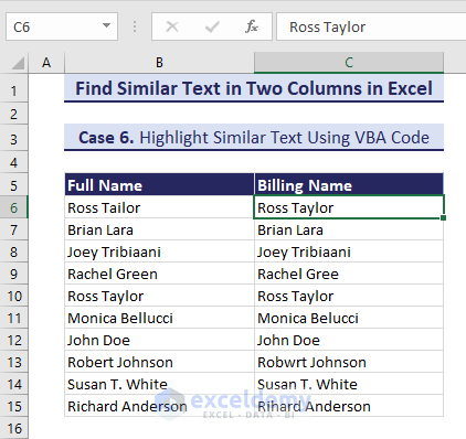
In the following image, you see two columns having similar names. Column E shows which names are exactly the same and which are not.

In this article, you will learn how to

• Find the same text in two columns side by side or in whole columns.
• Check if two columns have the same first or last words in their text string.
• Find the similarity of text in two columns by matching the first or last N characters.
• Find and extract words with the same prefix or suffix.
• Use VBA to similar text in two columns and highlight them.

Lastly, we have shown how to use the Find command to find similar text in the whole worksheet or workbook.

Method 1 – Find Exactly Same Text in Two Columns by IF Function (Compare Side by Side)

We have some names in two columns (B and C). Let’s compare B6 with C6, B7 with C7 and so on. If B6=C6, we will comment “Same” in cell E6. If B6≠C6, let’s use “Not Same”.

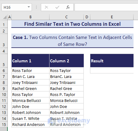
Follow these steps:

• Input this formula in cell E6:

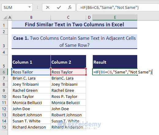
• Press Enter and you will get the output.

Ross Taylor and Ross Tailor do not match because Tailor and Taylor are not spelt the same.

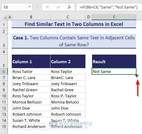
• Hover your mouse over the bottom right corner of cell E6, and you will find the Fill Handle icon.
• Double-click on the Fill Handle icon, which will copy the formula for the rest of the cells.

Read More: Formula to Find Duplicates in Excel

Method 2 – Check If a Text Is Found in Any of the Two Columns by Using Conditional Formatting

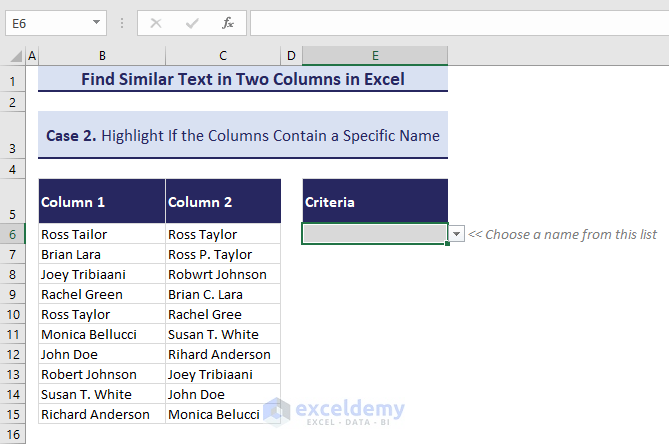
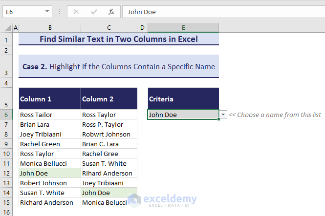
To check if a text is found in any of the two columns and highlight the cells with a color, let’s first set criteria in cell E6:

• In cell E6, I input a name, e.g., John Doe.

Then we will highlight the cells in two columns that have this name:

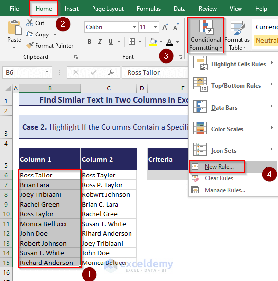
• Select all the values (B6:B15) of the first column.
• Go to the Home tab, click on the Conditional Formatting drop-down, and choose the New Rule option.
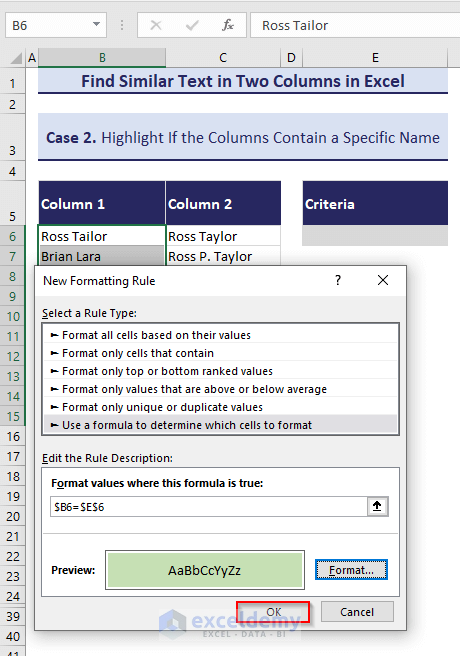
• The New Formatting Rule dialog box will open.

• In the New Formatting Rule dialog box, select Use a formula to determine which cells to format.
• Put the following formula in the formula box:

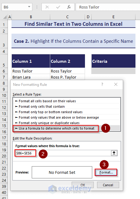
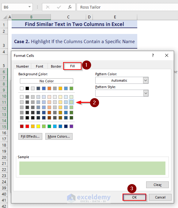
• Click on the Format button and the Format Cells dialog box will open.
• Go to Fill tab and choose a Background Color.
• Press OK.

• Click on the OK button in the New Formatting Rule dialog box to apply the changes.

• Repeat the same process to apply the Conditional Formatting in the second column.
• If we select the name John Doe from the drop-down, the names present in both columns will be highlighted with a light green color.

Read More: How to Find Duplicate Values Using VLOOKUP in Excel

Method 3 – Check If Two Columns Have Partially Same Text (Same First/Last Word)

In this section, we will show you how to find the texts in two columns that have the same first or last word.

For example, Ross Taylor and Ross Tailor are not exactly the same, but their first names have the same spelling. The similar concept applies to Robwrt Johnson and Robert Johnson—both have the same last names.

To match the first or last words in 2 columns, we have to use the LEFT and FIND functions (for the first word) or RIGHT and FIND functions (for the last word).

Case 1 – Check for Same First Word

Follow these steps:

• In cell E6, input this formula:

• Press Enter and then copy the formula down to all cells.

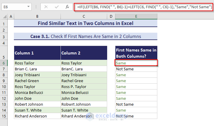
• We have applied conditional formatting to distinguish the matched and mismatched names.

Case 2 – Check for Same Last Word

Follow these steps:

• In cell E6, input this formula:

Here, RIGHT(B6,LEN(B6)-FIND(“^”,SUBSTITUTE(B6,” “,”^”,LEN(B6)-LEN(SUBSTITUTE(B6,””,””)))) returns the last names from cell B6 and other part returns the last name from cell C6.

If the last name of cell B6 equals the last name of cell C6, the IF function will return “Same.” Otherwise, it returns “Not Same”.

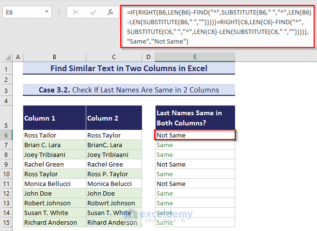
• Press Enter and copy the formula down to all cells and you find all the cells of the two columns that have the same last name.

Read More: How to Find Duplicates without Deleting in Excel 

Method 4 – Find Similar Text by Matching First/Last N Characters in Two Lists

To match the characters, we will use IFERROR and SEARCH functions with the LEFT or RIGHT functions.

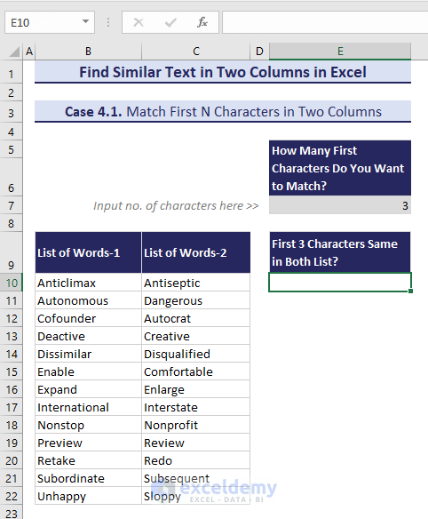
Case 1 – Match First N Characters

Consider the following dataset with two lists of words. We want to know whether pairs of words (i.e. one word from the first list and its corresponding word in the second) share the same N first characters.

Follow these steps:

• Put the number in cell E7. This is how many characters you want to match. Here, we have put 3.

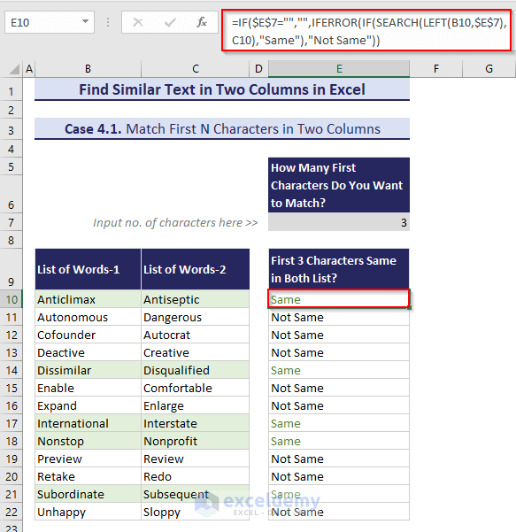
• In cell E10, input this formula:

• Copy the formula down.

After copying the formula in all cells, you’ll find all the rows where the first 3 characters are the same.

Case 2 – Match Last N Characters

Here, we’ll match the last N characters of the adjacent cells of the 2 columns. The rest of the setup is the same as in previous case.

Change the formula to:

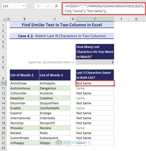
Read More: Excel Formula to Find Duplicates in One Column

Method 5 – Find and Extract Words with Same Prefix or Suffix

Sometimes you may need to find and extract words with the same prefix or suffix. You can do this by using the FILTER, TOCOL and other Excel functions.

Case 1 – Extract Words with Same Prefix

Let’s use the following dataset with the list of words in two columns.

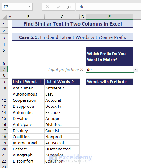
Follow these steps:

• Choose a prefix from the drop-down (we choose de). If you don’t make a drop-down, you can input manually.
• In cell E10, input this formula:

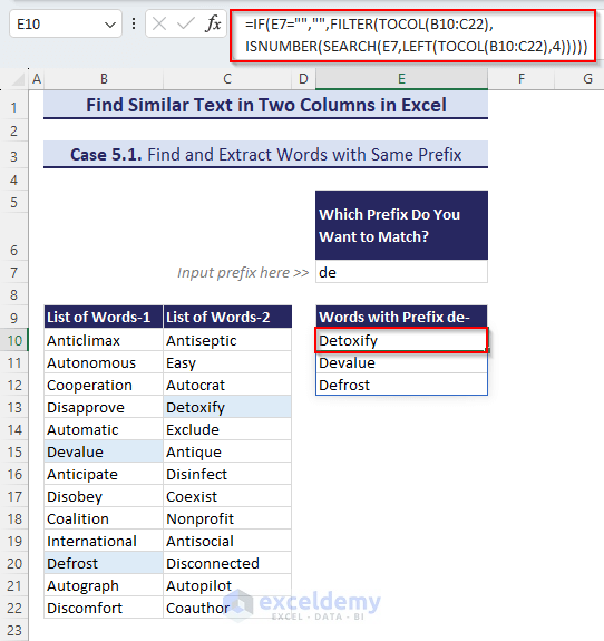
• Press Enter and you’ll get all the words with the prefix de in a single column.

Case 2 – Extract Words with Same Suffix

• The setup is similar for the first case, but the drop-down contains a list of suffixes (if you don’t make one, use manual input.
• Choose a prefix.
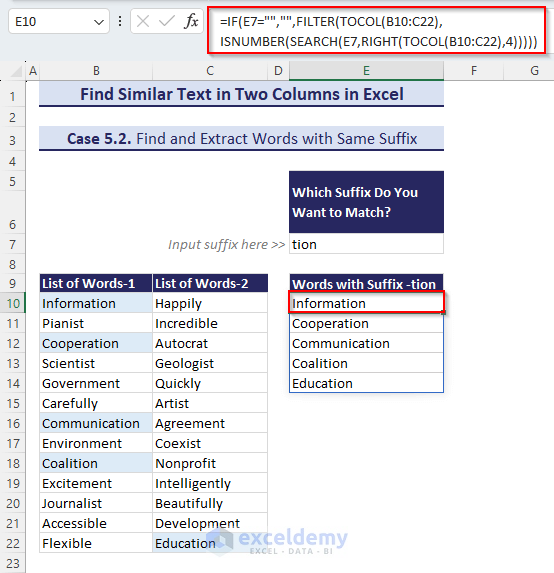
• In cell E10, input this formula:

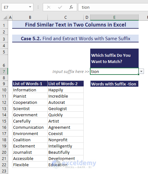
• After pressing Enter, you’ll get all the words with the suffix in a single column.

Read More: Find and Highlight Duplicates in Excel 

Method 6 – Use VBA to Find and Highlight Similar Text in Two Columns

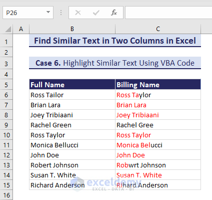
We’ll compare two columns and match text of each column from the left, then highlight the matched part of the 2nd string with a color. Let’s use the same dataset with names as before.

Follow these steps:

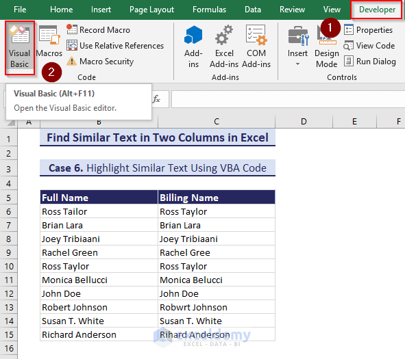
• Go to the Developer tab and click on the Visual Basic option. You can use the keyboard shortcut Alt + F11 to open the Visual Basic window directly.

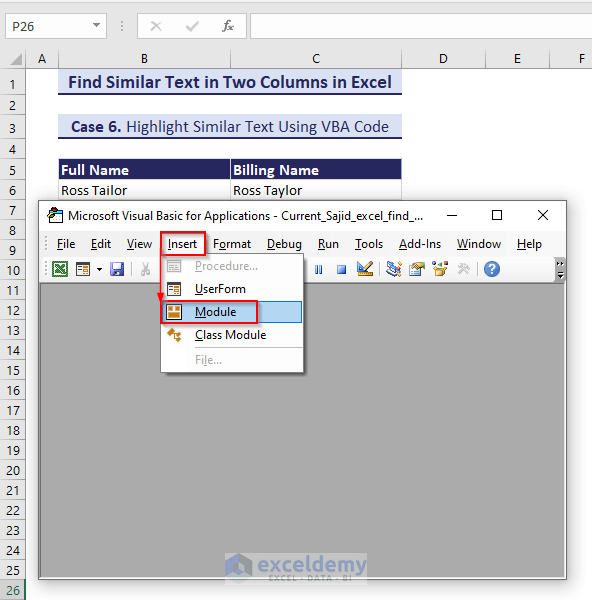
• Go to the Insert tab and click on the Module option. A new Module will open.

• Put the following code in the Module:

Sub highlight_similar_text()
On Error Resume Next
If ActiveWindow.RangeSelection.Count > 1 Then
Text = ActiveWindow.RangeSelection.AddressLocal
Else
Text = ActiveSheet.UsedRange.AddressLocal
End If
One:
Set Range1 = Application.InputBox("First Range:", "Exceldemy", Text, , , , , 8)
If Range1 Is Nothing Then Exit Sub
If Range1.Columns.Count > 1 Or Range1.Areas.Count > 1 Then
MsgBox "You select several columns ", vbInformation, "Exceldemy"
GoTo One
End If
Two:
Set Range2 = Application.InputBox("Second Range:", "Exceldemy", "", , , , , 8)
If Range2 Is Nothing Then Exit Sub
If Range2.Columns.Count > 1 Or Range2.Areas.Count > 1 Then
MsgBox "You select several columns ", vbInformation, "Exceldemy"
GoTo Two
End If
If Range1.CountLarge <> Range2.CountLarge Then
MsgBox "Selected ranges should be equal ", vbInformation, "Exceldemy"
GoTo Two
End If
Differ = (MsgBox("Select Yes for similar text, Select No for dissimilar text ", vbYesNo + vbQuestion, "Exceldemy") = vbNo)
Application.ScreenUpdating = False
Range2.Font.ColorIndex = xlAutomatic
For I = 1 To Range1.Count
Set FirstCell = Range1.Cells(I)
Set SecondCell = Range2.Cells(I)
If FirstCell.Value2 = SecondCell.Value2 Then
If Not Differ Then SecondCell.Font.Color = vbRed
Else
xLen = Len(FirstCell.Value2)
For J = 1 To xLen
If Not FirstCell.Characters(J, 1).Text = SecondCell.Characters(J, 1).Text Then Exit For
Next J
If Not Differ Then
If J <= Len(SecondCell.Value2) And J > 1 Then
SecondCell.Characters(1, J - 1).Font.Color = vbRed
End If
Else
If J <= Len(SecondCell.Value2) Then
SecondCell.Characters(J, Len(SecondCell.Value2) - J + 1).Font.Color = vbRed
End If
End If
End If
Next
Application.ScreenUpdating = True
End Sub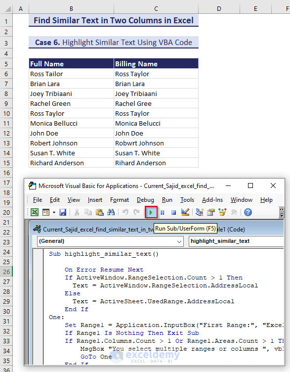

• Press the Run button to run the code and you’ll get an input box. You can also apply the keyboard shortcut F5 to run the code.
• Put the range of the first column in the box.

• Click OK and you’ll get another input box.
• Put the range of the second column in the box.

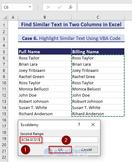
• Click OK and you’ll get a confirmation dialog box.

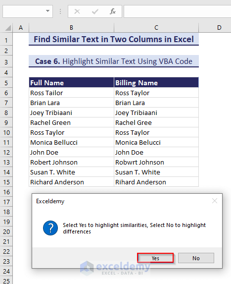
• Choose Yes to highlight the similarities in the second column.

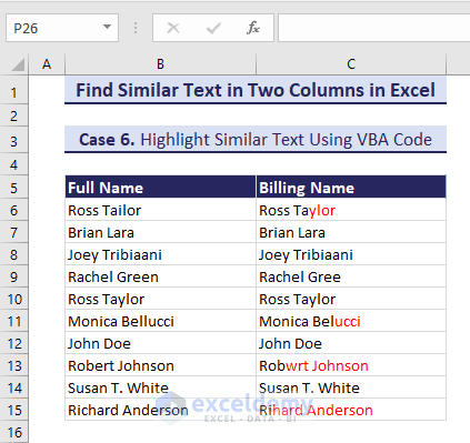
• Alternatively, select No to highlight the differences in the second column.

Read More: Find Duplicates in Two Columns in Excel 

How to Use the Find Command to Find Similar Text in Two Columns in Excel

You can perform both exact and partial match (with ampersand and question mark operator) through this Find command:

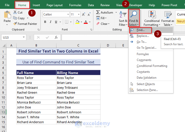
• Go to the Home tab, click on the Find & Select drop-down, and select the Find command. The Find and Replace dialog box will open. (The keyboard shortcut is Ctrl + F)

• We want to find all the similar text matches with Ross. So, put that in the search box.

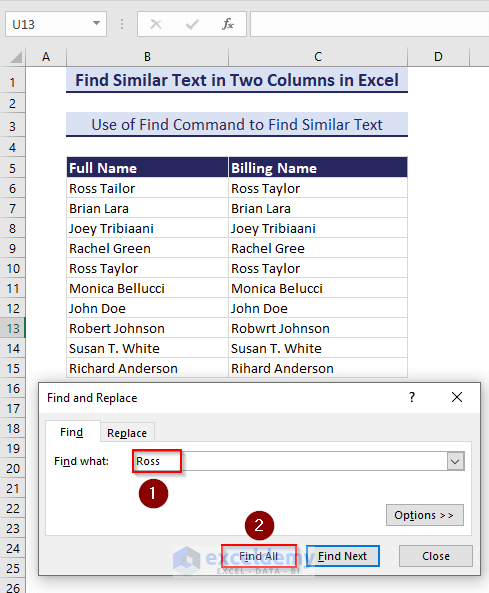
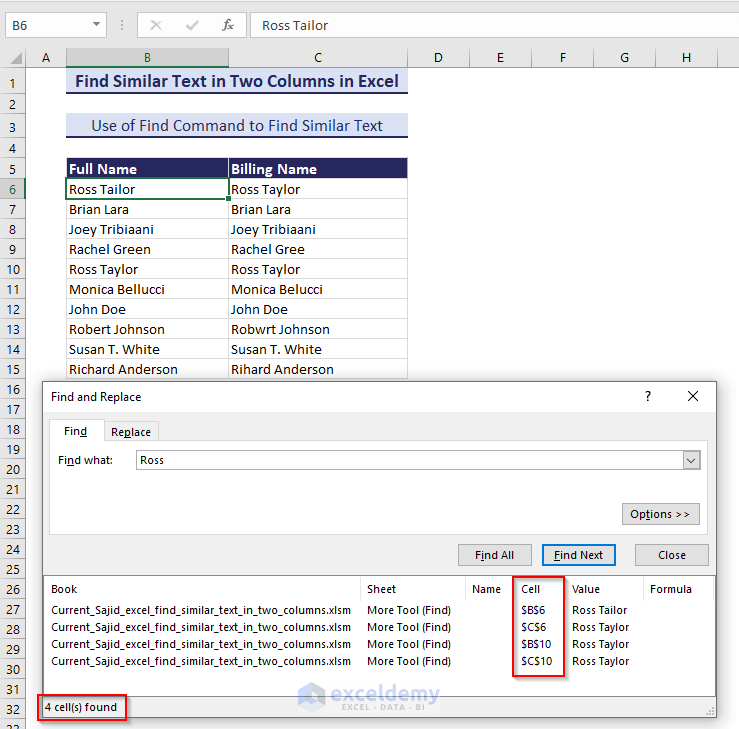
• Click on the Find All button and you’ll get the result. You can see the texts and their position that match with the search result.

• You can also do partial matching. Type R*T and you’ll get all the matching texts that have R in the starting position and T in the last position.

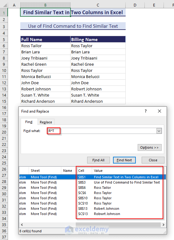
• Type R?T and you’ll get only two matching texts that have R in the starting position and T in the last position and have space in between them.

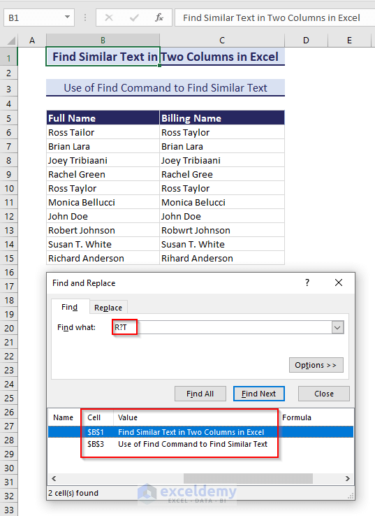
• If you click on any row of this list, it will take you to the respective cell.

Download Practice Workbook

Related Articles

• How to Find Duplicates in Excel Workbook
• How to Find Duplicates in Two Different Excel Workbooks

<< Go Back to Find Duplicates in Excel Column | Find Duplicates in Excel | Learn Excel