Latest Posts From Masum Mahdy

Data Entry Form in Excel: Knowledge Hub How to Create Data Entry Form in Excel How to Make an Excel Spreadsheet Look Like a Form How to Create an ...

Entering and Editing Data in Excel: Knowledge Hub How to Enable Editing in Excel How to Press Enter in Excel Without Changing Cells Making Same ...

Excel Sum with VLOOKUP: Knowledge Hub How to Sum All Matches with VLOOKUP in Excel Use VLOOKUP to Sum Multiple Rows in Excel How to Combine SUMIF ...

Excel Function Categories: Knowledge Hub Excel LOOKUP and Reference Functions Excel Date Functions Use of Excel Database Functions DGET, DAVERAGE, ...

A histogram is one kind of graph which we use to show frequency distribution within some prespecified ranges. These data ranges are called ‘bins’. The ...

Creating a named range in Excel is an easy task. But, if you want to make the named range dynamic so that whenever you add new data, the named range will ...

Multidimensional Scaling is a way to visually present the similarity between objects (brands, product attributes, etc.) in a 2-dimensional scale, i.e. a ...

Extrapolation is known as extending a current trend into the future or applying sample study findings to the entire population. In this article, we will show ...

To separate odd and even numbers: Method 1 - Combining the FILTER and the MOD Functions to Separate Odd and Even Numbers Steps: In C5, enter ...

In this article, you will learn how to fill in odd numbers in Excel. How to Fill Odd Numbers in Excel: 5 Suitable Examples 1. Use Fill Handle Tool to ...
![Can Excel DGET Return Multiple Records [See 4 Solutions]](https://www.exceldemy.com/wp-content/uploads/2022/12/excel-dget-multiple-records-1.png?v=1697451912)
The DGET function in Excel is a database function and is designed to return only one record. In case you have multiple matches and need to return multiple ...

Have you ever wondered how to apply the DGET function of Excel for multiple dynamic criteria? The DGET function of Microsoft Excel is one of the database ...

In this article, I will show how to calculate Mean Squared Error in Microsoft Excel with quick steps and clear illustrations. In practical life, we may have ...
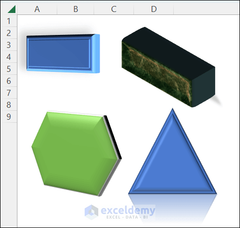
Wonder how to make a 3D drawing in Excel? You are in the right place! In this article, I have discussed how to construct a 3-dimensional drawing in Microsoft ...
Method 1 - Decide Which Accounting Method You Will Use Businesses primarily employ two accounting techniques: Accrual Accounting and Cash Accounting. ...
See Our Reviews at


Thank you for your compliment, David!
Please click on the following link for more examples of the INDEX-MATCH combo:
https://www.exceldemy.com/tag/index-match-excel/
You are welcome Rahul 🙂
Thanks Nelly for your appreciation.
You are welcome, G. 🙂
You are welcome, Shekhar! 🙂
Hi James, you have asked this on our forum too. We have answered the question in your thread. Please check it out and let us know if this helps you.
https://exceldemy.com/forum/threads/using-vba-to-pull-data-from-a-website-fails-on-a-lib-user32-statement.121/
Best regards.
Team ExcelDemy
That’s great 🙂
Thanks for your comment, Madison!
Thanks fhasim015! Glad to know that.
You are welcome Kannan!
You are most welcome Alok!
Glad to know, Sandeep!
-Mahdy
ExcelDemy team
Thanks Akash!
-Mahdy
ExcelDemy team
Hi Alex, it is a great pleasure for us to know that you are getting benefits from our content (and referring us to your friends too)!
Now, your answers:
1. No, you have to use the ROWS function too. Otherwise, you will not get the correct answer in other cases (your guess is true only for this particular set of data).
2. Yes. You are right. You have to use the COUNTIFS function. Use the following formula.
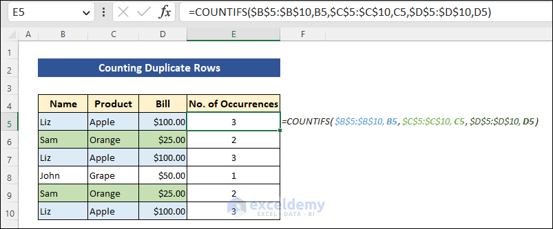
=COUNTIFS($B$5:$B$10,B5,$C$5:$C$10,C5,$D$5:$D$10,D5)If you have two columns only, remove the $D$5:$D$10,D5 part from the formula, i.e.
=COUNTIFS($B$5:$B$10,B5,$C$5:$C$10,C5)Now, copy the formula down. The output number will say how many times each row is repeated.
Regards
-Mahdy
(ExcelDemy Team)
Dear X,
Thank you so much for following the article. We can still see the Zoom option in the status bar and in the view tab as the author described in this article. So we cannot fully understand what your specific issue is. Would you please post your problem with a screenshot on our Excel Forum?
Regards
-ExcelDemy Team
Hi Anil, here is an easier and shorter formula for you. (FILTER function is available from Excel 2019)
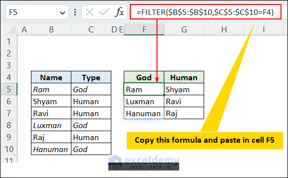
=FILTER($B$5:$B$10,$C$5:$C$10=F4)Do the following to your desired list.
>> Write “God” in cell F4 and “Human” in cell G4.
>> Copy the above formula and paste it into cell F5 (it will list God Names)
>> Similarly generate the Human Names. Just use G4 instead of F4 in the given formula.
Can you visualize what to do? Please let us know if this helps.
Regards
-ExcelDemy Team
Hi Shimrit, you are most welcome! We are glad to hear that it worked for you.
Regards
-ExcelDemy Team
Hi Haley,
We have updated the Excel workbook and added a new raw worksheet. So now you can practice from scratch. Stay with us always.
Regards
-ExcelDemy Team
Download File Link:
Practice Workbook
You may find this formula useful.
=SUM(FILTER(B2:S2,ISEVEN(COLUMN(B2:S2)))-FILTER(B2:S2,ISODD(COLUMN(B2:S2))))Just instead of B2:S2, put your own cell range.
Regards
-ExcelDemy Team
Hi ROD, we are really sorry for your experience, there is no Excel formula to move data from one cell to another actually. So we have revised the whole write-up. Thanks for your (Bill too) valuable feedback. We hope you will be with us in the coming days as well.
-ExcelDemy Team
Dear HEATHER, I guess you are facing the same problem as HANNAH. But we have rechecked the code, and applied it again, but have found no issue.
Can you please send us your problem with specific details? Here is our address: [email protected]
We have added the code explanation. Have a look at it and let us know if it can do any help regarding your problem. But the best will be to send your problem in detail with your Excel file. Thanks and regards.
-ExcelDemy Team
Hi Don. Thanks for letting us know about this. 🙂 We have updated the blog post. Regards
-ExcelDemy Team
Hi JIM, we are really sorry if these methods cannot help you. Yes, we agree with all of you that empty strings and blank cells are not the same in Excel. We have tried to show some ways to set cells to “seemingly blank” using Excel formulas.
Now, if you need to set cells to absolutely empty (nothing inside cells), sorry Excel formula cannot help you in this regard. But if seemingly blank is enough for you, these formulas work properly.
If you have a specific case, where you need to set cells to truly blank, then let us know at [email protected] with your problem-details and Excel file. We will definitely try to help.
Best regards.
-ExcelDemy Team
You are welcome, Henry. Yes, it’s possible. Please share your problem with details at [email protected]
Regards.
Hi AVINASH. Check your email for a sample file. I have used the INDIRECT function with the Data Validation command to make it.
Regards.
Hi GABOR! Please click on the following link to get a code that will help you to save selected worksheets in the list as PDF files in a suitable location.
https://www.exceldemy.com/vba-code-for-print-button-in-excel/#3_Apply_VBA_Code_to_Create_Print_Button_for_Selected_Sheets_in_Excel
Note that, you have to go through the first two steps of the first example in the given article. Then you can apply the code there. (We have mentioned it there also.)
Stay with us. Best regards.
Hi AKSHAY THAKKER! We hope you are well. It’s been 6 years since you posted this query here. We are extremely sorry for being so late in responding. Hope you would have had a solution to your problem somewhere by now. However, we are providing a solution to your question hoping that other readers might find it useful.
For example, we have created a 10×10 array using the following formula.
Look at the following image.
You must do two things before applying the formula.
First, place the numbers in the first row (row 1, i.e. row of A1) serially, and second, place them serially down the first column (column A). You can place them elsewhere, but in that case, you have to change the cell references in the array formula accordingly.
You can create any square array with your desired sequence (1,1,1,1;2,2,2,0;3,3,0,0;4,0,0,0) having any square dimension. However, if you want to change the sequence, you have to change the formula a bit.
Tip: Look into the greater than logic in the formula. You have to make the change here to create other sequences.
If there is any query, please let us know. You can also send us your problem at this address: [email protected]
You are welcome, Surya 🙂
You are welcome, Ahmad 🙂
Hi, Muhammad! Of course, you can do that. Check this out 🙂
https://www.exceldemy.com/excel-macro-to-copy-and-paste-from-one-worksheet-to-another/#9_VBA_Macro_to_Copy_and_Paste_Selected_Data_from_One_Sheet_to_Another_in_Excel
Hello Jay, thanks for your nice words. Please visit our blog for more array posts! We have written more posts like this time by time.
You are welcome, Surya! 🙂
Thank you so much, Ferreira. Visit our blog and explore more!
Hi Bill Coriell! Sorry for being late in reply. Maybe you were asking for the following article.
https://www.exceldemy.com/what-is-an-array-in-excel/
With regards
-ExelDemy team
Dear pat, sorry for replying late. Please send your file to [email protected] so that we can help. Thanks for commenting.
We are extremely sorry Hannah W. to know that you have faced this difficulty in applying our provided code! We have added the code explanation. Is your problem solved? Please let us know.
With regards
-ExcelDemy team
The code is perfectly working from our end, Goel! Can you please send your problem to this email: [email protected]?
Hi STACY! Thank you very much for your comment and appreciation. You can follow this article regarding your issue.
https://www.exceldemy.com/insert-date-picker-in-excel/
If this doesn’t help, please let us know. You can also send your problem with your Excel file to this email address: [email protected]
Thanks again for being with us.
With regards
-ExcelDemy team
You are welcome, Ruben! Please share your thoughts with us, too. Regards.
Hi Pete, you are right!
Variance= ABS(new value-original value)/original valueis the correct one.We are really grateful for your precious feedback. We have updated the Excel file and main content accordingly.
Best Regards.
-ExcelDemy team.
Hi Deepak!
The following formula can match two criteria and return multiple matches:
=INDEX($E$2:$E$14, SMALL(IF(COUNTIF($G$2, $C$2:$C$14)*COUNTIF($H$2, $D$2:$D$14), ROW($A$2:$E$14)-MIN(ROW($A$2:$E$14))+1), ROW(A1)), COLUMN(A1))Here,
$E$2:$E$14= Column to return matches$G$2 and $H$2= Criteria 1 and 2$C$2:$C$14and$D$2:$D$14= The columns of main data respective to criteria 1 and 2In a similar way, you can add any number of criteria.
Thank you for being with us.
Hi MAHENDRA TRIVEDI! You can use the following formula to compare two columns and return multiple matches in a single cell:
=TEXTJOIN(",",TRUE,IF(A5:A15=D5,B5:B15,""))Here,
A5:A15= Range for matching criteria
B5:B15 = Range of the values to return
D5= Lookup value
TRUE ignores all the empty cells.
Check the 3rd case of the following article to know more details.
hhttps://www.exceldemy.com/index-match-return-multiple-values-vertically/
Thanks for being with us. Best regards.
Hi CLÉMENTINE! You have to select the newly added data from the filter list first (mark the Select All box for that). Then the filter command will work as usual. Thanks!
Hi Stevoisiak! Hope you are doing well.
Suppose you have the following name in cell B5.
Mr. Brian Charles Lara
To extract all the parts of this name, use the following formulas.
To separate prefix:
=LEFT(B5,SEARCH(" ",B5)-1)To separate first name:
=MID(B5,SEARCH(" ",B5)+1,SEARCH(" ",B5,SEARCH(" ",B5)+1)-(SEARCH(" ",B5)+1))To separate middle name:
=MID(B5,SEARCH(" ",B5,SEARCH(" ",B5,1)+1)+1,SEARCH(" ",B5,SEARCH(" ",B5,SEARCH(" ",B5,1)+1)+1)-(SEARCH(" ",B5,SEARCH(" ",B5,1)+1)+1))To separate last name:
=RIGHT(B5,LEN(B5)-FIND("^",SUBSTITUTE(B5," ","^",LEN(B5)-LEN(SUBSTITUTE(B5," ","")))))You can check the following article too, to know more.
https://www.exceldemy.com/separate-first-middle-last-name-with-excel-formula/
Best Regards.
Hi DAVID BAKER! Hope you are well!
This article will help you to highlight specific data in cells.
https://www.exceldemy.com/highlight-specific-text-in-excel-cell-vba/
Best Regards.
Hi GEOFFREY! Your problem is not quite clear to us. However, if you simply copy and paste the cell contents, the hyperlinks will also be pasted. If this is not what you were expecting, then we would request you to elaborate on your issue. You can also send your Excel file to us through email. Thank you!
We appreciate your nice suggestion, ANTHONY! You can also see the following article to know about all the Paste Options in Excel.
https://www.exceldemy.com/paste-options-in-excel/
Thank you for being with us. 🙂
Hi Sara, the macro in #9 works fine on our part. Have you changed the Range(B5:D14) according to your dataset? If you have typed the range correctly, and still the macro is not working for the last row, please let us know.
Hi Rakesh! I hope this formula will do the task for you.
=TEXTJOIN("",TRUE,IFERROR((MID(A1,ROW(INDIRECT("1:"&LEN(A1))),1)*1),""))Here are more ways to extract just numbers from your data.
https://www.exceldemy.com/extract-only-numbers-from-excel-cell/