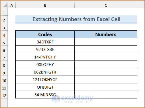
We have some codes including digits and letters where digits are present at the beginning. We’ll extract those digits.
Method 1 – Combining LEFT, SUM, LEN, and SUBSTITUTE Functions to Extract Numbers Only from the Beginning of Text in Excel Cell
Steps:
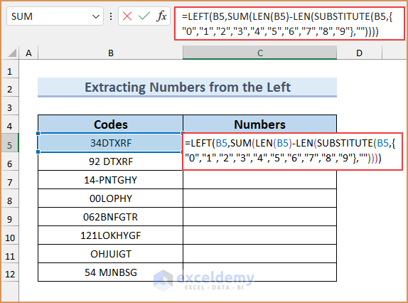
- Insert this formula in cell C5.
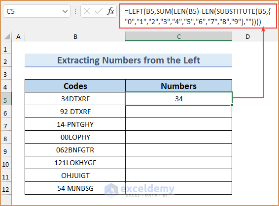
=LEFT(B5,SUM(LEN(B5)-LEN(SUBSTITUTE(B5,{"0","1","2","3","4","5","6","7","8","9"},""))))
- Press Enter.
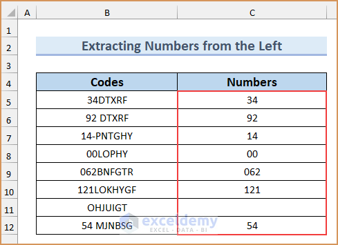
- Use the Fill Handle to autofill all other cells in column C.
Formula Breakdown
➤ SUBSTITUTE(B5,{“0”, “1”, “2”, “3”, “4”, “5”, “6”, “7”, “8”, “9”},””)
- The SUBSTITUTE function will find the digits (0-9) consecutively and, if found, it will replace that digit in cell B5 with an empty character every time. So, the function will return as- {“34DTXRF”, “34DTXRF”, “34DTXRF”, “4DTXRF”, “3DTXRF”, “34DTXRF”, “34DTXRF”, “34DTXRF”, “34DTXRF”, “34DTXRF”}.
➤ LEN(SUBSTITUTE(B5,{“0”, “1”, “2”, “3”, “4”, “5”, “6”, “7”, “8”, “9”},””))
- The LEN function determines the number of characters in a string. So, here, the LEN function will count all the characters individually found in the texts through the SUBSTITUTE function. The resultant values will be here in our case – {7,7,7,6,6,7,7,7,7,7}.
➤ LEN(B5)-LEN(SUBSTITUTE(B5,{“0”, “1”, “2”, “3”, “4”, “5”, “6”, “7”, “8”, “9”},””)))
- This part is the subtraction from the number of characters in cell B5 to all other numbers of characters found individually in the previous section of the formula. So, here the resultant values will be – {0,0,0,1,1,0,0,0,0,0}.
➤ SUM(LEN(B5)-LEN(SUBSTITUTE(B5,{“0”, “1”, “2”, “3”, “4”, “5”, “6”, “7”, “8”, “9”},””)))
- The SUM function will then simply sum all the subtracted values found & so the result will be here, 2 (0+0+0+1+1+0+0+0+0+0).
➤ =LEFT(B5, SUM(LEN(B5)-LEN(SUBSTITUTE(B5,{“0”, “1”, “2”, “3”, “4”, “5”, “6”, “7”, “8”, “9”},” ))))
- The LEFT function will return the values with an exact number of characters from the left found in the previous section of the formula. As we got the sum value as 2, the LEFT function here will return only 34 from the text 34DTXRF.
Method 2 – Joining Excel RIGHT, MIN, and SEARCH Functions to Extract Only Numbers from the Right Side of Text in the Cell
Steps:
- Insert the following formula in the cell C5.
=RIGHT(B5,LEN(B5) - MIN(SEARCH({0,1,2,3,4,5,6,7,8,9}, B5&"0123456789")) +1)
- Press Enter and then use the Fill Handle to autofill the rest of the cells.
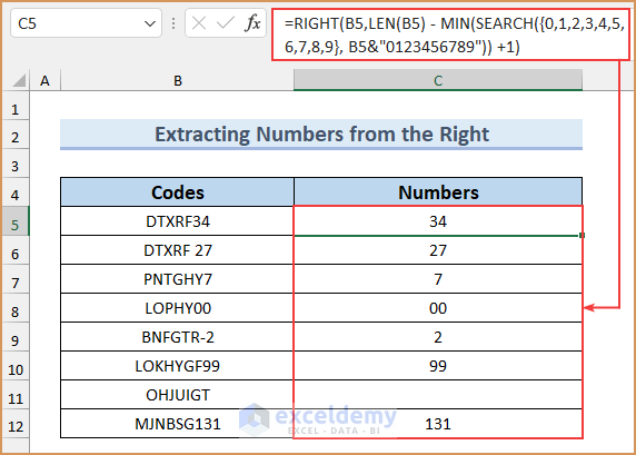
Formula Breakdown
➤ B5&”0123456789″
- We’re concatenating values in the B5 cell with 0123456789 by using ampersand (&) between them and we’ll get the resultant value as DTXRF340123456789.
➤ SEARCH({0,1,2,3,4,5,6,7,8,9}, B5&”0123456789″)
- The SEARCH function will search for all the digits (0-9) one by one in the resultant value obtained from the previous section and will return the positions of those 10 digits in the characters of DTXRF340123456789. So, here our resultant values will be {8,9,10,6,7,13,14,15,16,17}.
➤ MIN(SEARCH({0,1,2,3,4,5,6,7,8,9}, B5&”0123456789″))
- The MIN function is used to find the lowest digit or number in an array. So, here the minimum or lowest value will be 6 from the array {8,9,10,6,7,13,14,15,16,17} found in the preceding section of the formula.
➤ LEN(B5) – MIN(SEARCH({0,1,2,3,4,5,6,7,8,9}, B5&”0123456789″)) +1)
- The number of characters in B5 will be found by the LEN function. Then, it’ll subtract the value 6(found in the last section) and then return the result by adding 1. Here in our case, the resultant value will be 2 (7-6+1).
➤ RIGHT(B5,LEN(B5) – MIN(SEARCH({0,1,2,3,4,5,6,7,8,9}, B5&”0123456789″)) +1)
- The RIGHT function will return the specified number of characters from the last or right side of a string. The RIGHT function will show the last 2 characters from cell B5, and that’ll be 34.
Method 3 – Merging Excel TEXTJOIN, IFERROR, and INDIRECT Functions to Extract Numbers from Any Part of a Text String
Steps:
- Insert the formula in your destination cell as follows-
=TEXTJOIN("",TRUE,IFERROR((MID(B5,ROW(INDIRECT("1:"&LEN(B5))),1)*1),""))
- If you’re using Excel 2016 or a later version press Enter, otherwise press Ctrl + Shift + Enter to get the result for this array formula.
- Autofill other cells using the Fill Handle.
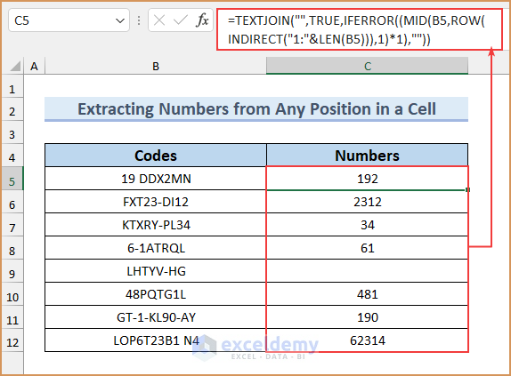
Formula Breakdown
➤ INDIRECT(“1:”&LEN(B5))
- The INDIRECT function is used to store an array of cell values as a reference text. Here the ampersand (&) command concatenates the length of the characters of cell B5 with incomplete range syntax (1:).
- The INDIRECT function will store all the numbers between 1 and the length of the characters in cell B5 as a reference text.
➤ ROW(INDIRECT(“1:”&LEN(B5)))
- The ROW function usually tells the row number of a cell. But here in the INDIRECT function, as no reference cell has been mentioned, in this case, the ROW function will extract all the values or numbers from the reference texts stored in the INDIRECT function.
- For the cell B5, the resultant values through these ROW and INDIRECT functions will be- {1;2;3;4;5;6;7;8;9}.
➤ (MID(B5,ROW(INDIRECT(“1:”&LEN(B5))),1))
- The MID function will let you determine the characters from the middle of a text string, given a starting position & length.
- For all 9 positions found in the previous section, the MID function now will show all the characters one by one for each position & thus will return the values as {“1”; “9”;” “; “D”; “D”; “X”; “2”; “M”; “N”}.
➤ IFERROR((MID(B5,ROW(INDIRECT(“1:”&LEN(B5))),1)*1),””)
- The IFERROR is a logical function that will determine if a string is a number or something else. If it does not identify a string with numbers or digits, then it’ll return the value with a defined text command.
- In our case, all the values found in the last section will be multiplied by 1, and when the results are returned as value errors for letters or text values that cannot be multiplied, their IFERROR function will convert the errors into empty strings. So, our resultant values will be then- {1;9;””;””;””;””;2;””;””}.
➤ =TEXTJOIN(“”,TRUE,IFERROR((MID(B5,ROW(INDIRECT(“1:”&LEN(B5))),1)*1),””))
- This function is used to concatenate or join two strings with a specified delimiter.
- The resultant values we have found in the preceding section will now be joined together alongside this TEXTJOIN function. We’ll get the number 192.
Method 4 – Nesting Multiple Functions to Extract Only Numbers from Excel Cell
- Insert this formula in cell C5.
=IF(SUM(LEN(B5)-LEN(SUBSTITUTE(B5, {"0","1","2","3","4","5","6","7","8","9"}, "")))>0, SUMPRODUCT(MID(0&B5, LARGE(INDEX(ISNUMBER(--MID(B5,ROW(INDIRECT("$1:$"&LEN(B5))),1))* ROW(INDIRECT("$1:$"&LEN(B5))),0), ROW(INDIRECT("$1:$"&LEN(B5))))+1,1) * 10^ROW(INDIRECT("$1:$"&LEN(B5)))/10),"")
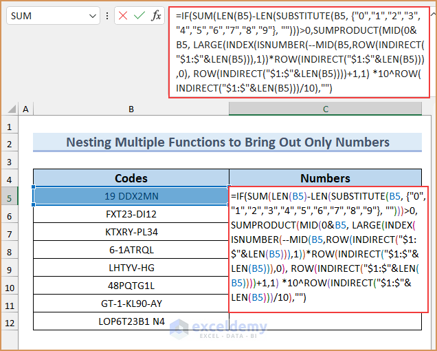
- Press Enter and use AutoFill.
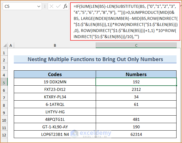
Formula Breakdown
Before starting the breakdown of this massive & compact formula, we can separate it into some parts:
=IF(A>0, SUMPRODUCT(B1*C1, B2*C2, ……….BnCn),””)
This syntax means if A is greater than 0, then all the products of Bn and Cn will sum up to the final result. And if A is not greater than 0 then the result will return as an empty or blank cell.
- A = SUM(LEN(B5)-LEN(SUBSTITUTE(B5, {“0”, “1”, “2”, “3”, “4”, “5”, “6”, “7”, “8”, “9”}, “
- B = MID(0&B5, LARGE(INDEX(ISNUMBER(–MID(B5,ROW(INDIRECT(“$1:$”&LEN(B5))),1))* ROW(INDIRECT(“$1:$”&LEN(B5))),0), ROW(INDIRECT(“$1:$”&LEN(B5))))+1,1)
- C = 10^ROW(INDIRECT(“$1:$”&LEN(B5)))/10),””
Breakdown of Part A = SUM(LEN(B5)-LEN(SUBSTITUTE(B5, {“0”, “1”,”2″,”3″,”4″,”5″,”6″,”7″,”8″,”9″}, “”
➤ SUBSTITUTE(B5, {“0″,”1″,”2″,”3″,”4″,”5″,”6″,”7″,”8″,”9”}, “”)
- The SUBSTITUTE function will find all digits (0-9) one by one in the text 19 DDX2MN each time and will replace those digits with an empty string in the positions of the digits.
- Thus the resultant values in an array will be- {“19 DDX2MN”,”9 DDX2MN”,”19 DDXMN”,”19 DDX2MN”,”19 DDX2MN”,”19 DDX2MN”,”19 DDX2MN”,”19 DDX2MN”,”19 DDX2MN”,”1 DDX2MN”}.
➤ LEN(SUBSTITUTE(B5, {“0″,”1″,”2″,”3″,”4″,”5″,”6″,”7″,”8″,”9”}, “”))
- The LEN function will now count the number of characters in all string values obtained from the previous section. So, this function will return as- {9,8,8,9,9,9,9,9,9,8}.
➤ LEN(B5)-LEN(SUBSTITUTE(B5, {“0″,”1″,”2″,”3″,”4″,”5″,”6″,”7″,”8″,”9”}, “”))
- Now in this part of the formula, a number of characters in cell B5 will subtract all the numbers found in the preceding section. The resultant values will be then- {0,1,1,0,0,0,0,0,0,1}.
➤ SUM(LEN(B5)-LEN(SUBSTITUTE(B5, {“0″,”1″,”2″,”3″,”4″,”5″,”6″,”7″,”8″,”9”}, “”)))
- With the help of the SUM function, the values inside the array found in the last section will add up to 3 (0+1+1+0+0+0+0+0+0+1).
- According to the first part of our formula, A>0 (3>0). We’ll move to the next part of the breakdown.
Breakdown of Part B = MID(0&B5, LARGE(INDEX(ISNUMBER(–MID(B5,ROW(INDIRECT(“$1:$”&LEN(B5))),1))* ROW(INDIRECT(“$1:$”&LEN(B5))),0), ROW(INDIRECT(“$1:$”&LEN(B5))))+1,1)
➤ INDIRECT(“$1:$”&LEN(B5))
- The INDIRECT function here will store the string values as a reference to the array. Inside the parenthesis, the ampersand (&) command will join the number of characters found in cell B5 with the Range of cells’ syntax. It means that from 1 to the number of characters defined, each will be stored as an array reference.
➤ ROW(INDIRECT(“$1:$”&LEN(B5)))
- This ROW function will pull out all the numbers from the array and the resultant values for cell B5 will be- {1;2;3;4;5;6;7;8;9}.
➤ MID(B5,ROW(INDIRECT(“$1:$”&LEN(B5))),1)
- The MID function will express all the characters from cell B5 based on all the positions found as numbers in the previous section. So, the extracted values will be found after this part- {“1″;”9″;” “;”D”;”D”;”X”;”2″;”M”;”N”}.
➤ ISNUMBER(–MID(B5,ROW(INDIRECT(“$1:$”&LEN(B5))),1))
- As ISNUMBER is a logical function, it’ll determine individually if the values found in the preceding section are number strings or not. If yes, then it’ll return as TRUE, otherwise, it’ll display as FALSE.
- In our case, the result will be- {TRUE;TRUE;FALSE;FALSE;FALSE;FALSE;TRUE;FALSE;FALSE}.
➤ INDEX(ISNUMBER(–MID(B5,ROW(INDIRECT(“$1:$”&LEN(B5))),1))*ROW(INDIRECT(“$1:$”&LEN(B5))),0)
- If you notice inside the above function, a double-hyphen, known as Double Unary, has been used. It is used to convert all logical values into number strings- 1(TRUE) or 0(FALSE). Now, the INDEX function will return this result as- {1;1;0;0;0;0;1;0;0}.
- After that, the resultant values will be multiplied by the values obtained from the ROW function inside the array and the outcome will be- {1;2;0;0;0;0;7;0;0}.
➤ LARGE(INDEX(ISNUMBER(–MID(B5,ROW(INDIRECT(“$1:$”&LEN(B5))),1))*ROW(INDIRECT(“$1:$”&LEN(B5))),0), ROW(INDIRECT(“$1:$”&LEN(B5))))
- The LARGE function will now rearrange the largest values from the array according to the positions based on the numbers found in the ROW functions. & our resultant values for this section of the formula will be- {7;2;1;0;0;0;0;0;0}.
➤ MID(0&B5, LARGE(INDEX(ISNUMBER(–MID(B5,ROW(INDIRECT(“$1:$”&LEN(B5))),1))*ROW(INDIRECT(“$1:$”&LEN(B5))),0), ROW(INDIRECT(“$1:$”&LEN(B5))))+1,1)
- This part of the function will concatenate 0 with the texts in cell B5. Then it’ll add 1 individually with all the numbers found in the last section and show the characters from B5 cell based on the defined number positions.
- Our outcome from this section will be- {“2″;”9″;”1″;”0″;”0″;”0″;”0″;”0″;”0”}.
Breakdown of Part C = (10^ROW(INDIRECT(“$1:$”&LEN(B5)))/10),””)
- This part will determine the powers of 10 & store them inside the array. The digits of the powers are the numbers found from the ROW function previously.
- This part of the formula will return the values as- {1;10;100;1000;10000;100000;1000000;10000000;100000000}.
Multiplication of Bn and Cn
- The resultant values from the last two major breakdowns of B and C will now be multiplied inside the array. Then the products found from the multiplications will be- {2;90;100;0;0;0;0;0;0}.
- The SUMPRODUCT function will sum these values found in the array. So, our final outcome will be 192 (2+90+100+0+0+0+0+0+0), which is the extracted numbers from cell B5.
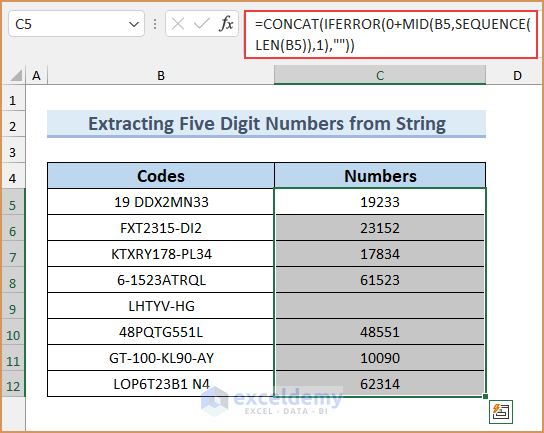
Method 5 – Combining Excel CONCAT and SEQUENCE Functions to Extract Five Digit Numbers Only from Cell String
Steps:
- Select the cell range C5:C12.
- Insert the following formula.
=CONCAT(IFERROR(0+MID(B5,SEQUENCE(LEN(B5)),1),""))
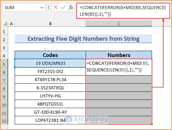
- Press Ctrl + Enter.
Formula Breakdown
- LEN(B5)
- Output: 11.
- This function returns the length of the string.
- SEQUENCE(11)
- Output: {1;2;3;4;5;6;7;8;9;10;11}.
- This function returns the first eleven numbers.
- MID(B5,{1;2;3;4;5;6;7;8;9;10;11},1)
- Output: {“1″;”9″;” “;”D”;”D”;”X”;”2″;”M”;”N”;”3″;”3″}.
- Using this part, we are getting the individual characters from the string.
- 0+{“1″;”9″;” “;”D”;”D”;”X”;”2″;”M”;”N”;”3″;”3″}
- Output: {1;9;#VALUE!;#VALUE!;#VALUE!;#VALUE!;2;#VALUE!;#VALUE!;3;3}.
- When we add zero with a string, it will return an error.
- IFERROR({1;9;#VALUE!;#VALUE!;#VALUE!;#VALUE!;2;#VALUE!;#VALUE!;3;3},””)
- Output: {1;9;””;””;””;””;2;””;””;3;3}.
- We are getting blank for all error values.
- CONCAT({1;9;””;””;””;””;2;””;””;3;3})
- Output: 19233.
- We are adding all the values to extract five digit numbers only.
Method 6 – Using Excel Flash Fill to Extract Numbers Only Within a Cell Range
Steps:
- Type the numbers manually in cell C5.
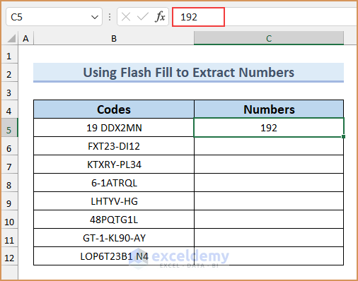
- Start typing the numbers from cell B6 to cell C6 and Excel will automatically recognize the pattern.
- Press Enter.
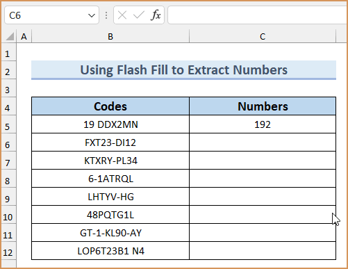
Notes: This method has some drawbacks, which is why it’s not recommended for all cases when you need to extract numbers from text strings. The Flash Fill usually follows a pattern from the cells in a column or a range. The first 2 or 3 extractions or calculations have to be done manually to help Excel absorb the common pattern of the resultant values. But sometimes, it does not follow the exact pattern we need and, thereby, it’ll follow its own pattern and give you a mismatched result.
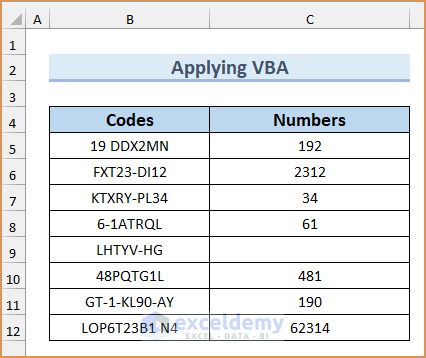
Method 7 – Applying VBA Code to Extract Only Numbers from an Excel Cell
Steps:
- Press Alt + F11 to open the VBA window.
- From the Insert tab, select Module. A new module window will appear.
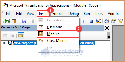
- Inside the module, paste the following code.
Option Explicit
Sub ExtractNumbersOnly()
    Dim CellValue As Range
    Dim InBx1 As Range
    Dim InBx2 As Range
    Dim NumChar As Integer
    Dim StartChar As Integer
    Dim XtrNum As String
    Dim DBxName1 As String
    Dim DBxName2 As String
    Dim Iteration As Integer
    DBxName1 = "Input Data Selection"
    DBxName2 = "Output Cell Selection"
    Set InBx1 = Application.InputBox("Input Range of Text Cells:", _
    DBxName1, "", Type:=8)
    If TypeName(InBx1) = "Nothing" Then Exit Sub
    Set InBx2 = Application.InputBox("Select Output Cells:", _
    DBxName2, "", Type:=8)
    If TypeName(InBx2) = "Nothing" Then Exit Sub
    Iteration = 0
    XtrNum = ""
    For Each CellValue In InBx1
        Iteration = Iteration + 1
        NumChar = Len(CellValue)
        For StartChar = 1 To NumChar
            If IsNumeric(Mid(CellValue, StartChar, 1)) Then
            XtrNum = XtrNum & Mid(CellValue, StartChar, 1)
            End If
        Next StartChar
    InBx2.Item(Iteration) = XtrNum
    XtrNum = ""
    Next CellValue
End Sub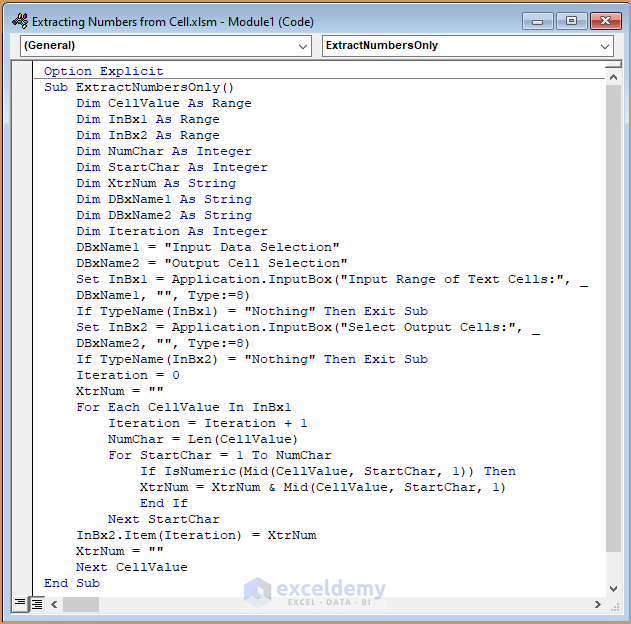
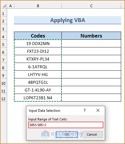
- Press F5 to execute the code. A dialog box named Input Data Selection will appear.
- Select all the text cells (i.e. B5:B12) and press OK.
- Another dialog box named Output cell Selection will appear. Select a cell or range of cells to see the output data or values. We put C5:C12 and pressed Enter.
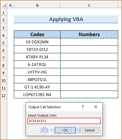
- You’ll see the extracted numbers from the texts.
VBA Code Breakdown
➤ Declaring Parameters
Option Explicit
Sub ExtractNumbersOnly()
    Dim cellValue As Range
    Dim InBx1 As Range
    Dim InBx2 As Range
    Dim NumChar As Integer
    Dim StartChar As Integer
    Dim XtrNum As String
    Dim DBxName1 As String
    Dim DBxName2 As String
    Dim Iteration As Integer
    DBxName1 = "Input Data Selection"
DBxName2 = "Output cell Selection"- We’re declaring all our parameters as integers, string values, or ranges of cells. Then we are giving the names of our dialogue boxes with “Input Data Selection” and “Output cell Selection”.
➤ Defining the Types of Inputs & Outputs for Dialogue Boxes
    Set InBx1 = Application.InputBox("Input Range of Text Cells:", _
    DBxName1, "", Type:=8)
    If TypeName(InBx1) = "Nothing" Then Exit Sub
    Set InBx2 = Application.InputBox("Select Output Cells:", _
    DBxName2, "", Type:=8)
    If TypeName(InBx2) = "Nothing" Then Exit Sub
    Iteration = 0
XtrNum = ""- We’re defining the parameters and their types for the dialogue boxes. Here, adding Type:=8 means the input and output data will consist of reference cells or a range of cells.
- We’re also defining that if input data is not found, then the subroutine will stop. By mentioning this macro, the subroutine will not break down for missing data, but rather it’ll stop functioning.
➤ Combining the Functions Inside the Code Loops for Iterations
For Each cellValue In InBx1
        Iteration = Iteration + 1
        NumChar = Len(cellValue)
        For StartChar = 1 To NumChar
            If IsNumeric(Mid(cellValue, StartChar, 1)) Then
            XtrNum = XtrNum & Mid(cellValue, StartChar, 1)
            End If
        Next StartChar
    InBx2.Item(Iteration) = XtrNum
    XtrNum = ""
    Next cellValue
End Sub- This is the most crucial part where we’re applying the functions or formulas that we need to assign to the texts to find the resultant values from the strings.
- VBA has built-in commands to use For or While loops where iteration for each and every detail in a text string can be executed without any hassle.
Download the Practice Workbook
<< Go Back to Separate Numbers Text | Split | Learn Excel
Get FREE Advanced Excel Exercises with Solutions!

This is excellent, how to sum each numbers from formula output like in B5 cell if output is 192 then sum 19+2
Thanks for your feedback. You have to use another formula to do that.
Semi-Qualifié 3 = SQ3
Semi-Qualifié 1 = SQ1
Manœuvre Spécialisé = MS
what is formula to simplyfy the words each first letter and combine like =
Hello Theva,
Glad that you shared your query. As per your given example, if you want to simplify the first letter of each word along with numbers, apply this simple VBA code.
Function ExtractFirstLetters(rng As Range) As StringDim arryDim X As Longarry = VBA.Split(rng, " ")If IsArray(arry) ThenFor X = LBound(arry) To UBound(arry)ExtractFirstLetters = ExtractFirstLetters & Left(arry(X), 1)Next XElseExtractFirstLetters = Left(arry, 1)End IfEnd FunctionNote that, if the words in your dataset are separated by Hyphens (–) then insert this line in the code
arry = VBA.Split(rng, "-")Instead of this,
arry = VBA.Split(rng, " ")I hope this will solve your problem. Let us know your feedback.
Regards,
Guria
ExcelDemy.
thank you so much
Dear Yasin,
You are most welcome.
Regards
ExcelDemy
Hello:
not work in my case since I need the minimum value in the same cell which si something like this:
Functional Test.: 4
In- Circuit Test: 4
Inspection, Visual: 7
Run-in Test: 4
Hello OLIVER,
I hope you are doing well. Thank u for your query. Well, you can use the below formula to extract only the minimum value in the same cell.
=MIN(IFERROR(VALUE(MID($B$4:$B$8, FIND(":", $B$4:$B$8) + 1, LEN($B$4:$B$8))), ""))Note: Change the range (B4:B8) according to your dataset.
Hope this information will help you. Please let us know if there is any further query in the comment section.
Best Regards,
Afrina Nafisa
Exceldemy
Thank you for providing these solutions! I get an error when I use the 3rd option, specifically when using the asterisk with “1”: textjoin(“”,true,iferror((mid([cellref],row(indirect(“1:”&LEN([cellref]))),*1),””))
Any tips?
Hello ScubaCamper,
Thanks for your appreciation. You are getting the error with asterisk because your formula attempts to multiply by 1 (*1) directly within the MID function’s parameters, that is not correct. You need to apply the multiplication outside of the MID function but within the array operation.
Please try this formula:
=TEXTJOIN(“”, TRUE, IFERROR(MID(B5, ROW(INDIRECT(“1:” & LEN(B5))), 1)* 1, “”))
In your formula style the formula would be: textjoin(“”,true,iferror((mid([cellref],row(indirect(“1:”&LEN([cellref]))),1)*1),””))
The purpose of multiplying by 1 (*1) in Excel formulas often is to convert text numbers to actual numeric values.
Regards
ExcelDemy
Hello, thankyou for putting this tutorial together.
How would I do this including decimal points? and if I had separate numbers in-between each string is there a way to send them to different columns?
Regards,
Harry
Hello Harry Ingram
Thanks for such an interesting comment. You wanted to extract numbers even if there are decimal points. Additionally, if there are more numbers, you want to put them in different columns. I have come up with a solution using several Excel VBA User-defined functions.
SOLUTION Overview:
To do so, follow these steps:
I have also attached the solution workbook; good luck.
DOWNLOAD SOLUTION WORKBOOK
Regards
Lutfor Rahman Shimanto
Excel & VBA Developer
ExcelDemy
Hello Harry Ingram,
You can use this formula to extract only the numbers, including the decimal point.
=TEXTJOIN(“”, TRUE, IFERROR(IF(ISNUMBER(SEARCH(MID(B5, ROW(INDIRECT(“1:” & LEN(B5))), 1), {“0″,”1″,”2″,”3″,”4″,”5″,”6″,”7″,”8″,”9″,”.”})), MID(B5, ROW(INDIRECT(“1:” & LEN(B5))), 1), “”), “”))
Feel free to download the Excel file from the link below, you’ll find examples of the formula.
Excel file: Extract Decimal Point Numbers
Regards,
ExcelDemy