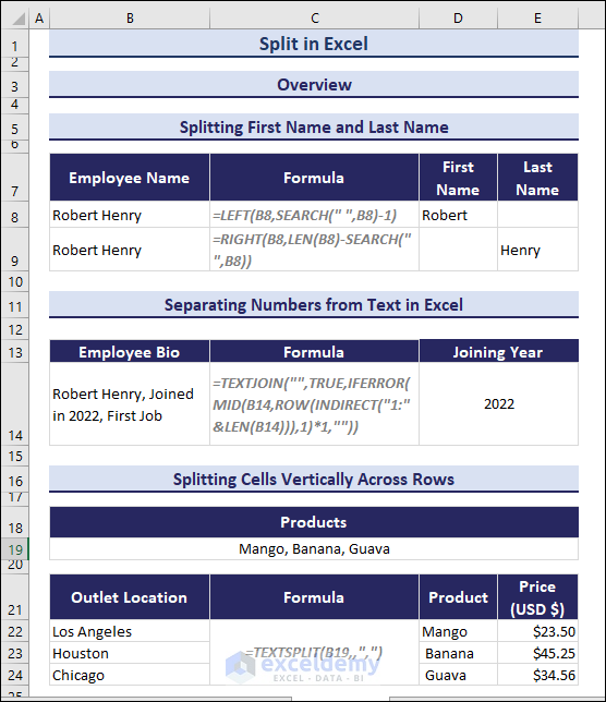
How to Split in Excel (Text, Numbers, Cells & Columns)

The overview shows the summary of splitting first and last names, separating numbers from text, and splitting cells vertically across rows. Here, the C column shows the formula to execute all these methods to split in Excel.

⏷Apply Excel Features to Split in Excel
⏵Using Text to Column Wizard
⏵Applying the Flash Fill Option
⏷Use Text Functions to Split Names
⏵Splitting First Name and Last Name
⏵Splitting First Name, Middle Name, and Last Name
⏷Applying TEXTSPLIT Function to Split Cells Across Columns and Rows
⏵Split Cells Horizontally Across Columns
⏵Split Cells Vertically Across Rows
⏷Separate Numbers from Text in Excel
⏷Split Merged Cells into Multiple Columns
⏷Split Cells Ignoring Missing Values
⏷Split Columns Using Power Query
⏷Apply VBA Macro to Split Cells

Part 1 – How to Apply Excel Features to Split in Excel

Method 1.1 – Using the Text to Column Wizard

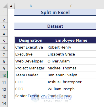
The dataset contains the full name Robert Henry. We will split the text of Employee Name into two columns and get the first name, Robert, and the second name, Henry, in individual cells.

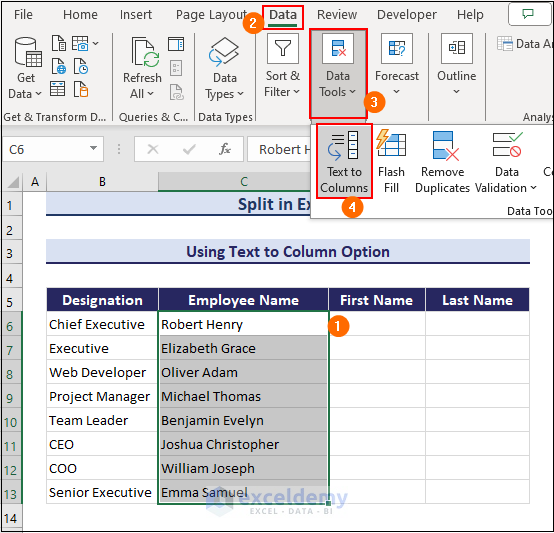
Select the cell range C6:C13 and go to the Data tab.
Choose Data Tools and select the Text to Columns option to get the Convert Text to Column Wizard dialog box.

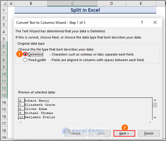
Select Delimited and click on the Next button to complete the first step.

Check Space and click on the Next button to complete the second step.

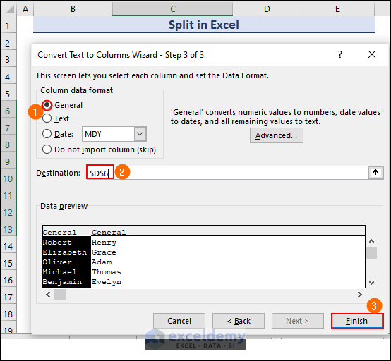
Go to the third step and select General from the Column data format.
Select cell D6 in the Destination field and click on the Finish button to complete the total process.
We have selected D6 to get the output on this cell.

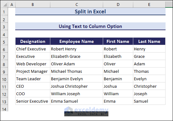
Here’s the output after splitting all cells using the Text to Column Wizard feature.

Method 1.2 – Applying Flash Fill

Write the first name in cell D6 and drag down the Fill handle to copy the name up to cell D13.
The Auto Fill option will pop up. Select Flash Fill from the drop-down menu of the Auto Fill option as below.
Repeat the same process by writing the last name in cell E6 and dragging down.

Note: Be careful about the consistency of your data. This method works because the pattern of the data is the same. This time, you only need the first and last names in every situation. If the pattern of the data is not the same, you can’t use the Flash Fill feature.

Part 2 – How to Use Text Functions to Split Name

Method 2.1 – Splitting the First Name and Last Name

We have a full name in C6 that we need to split between D6 and E6. The names are divided by a space.
Enter the following formula in cell D6 and drag the Fill Handle to the cell D13 to copy the formula.

=LEFT(C6,SEARCH(" ",C6)-1)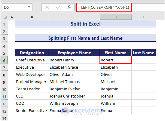

Enter the following formula in cell E6 and apply it to get the last name as an output, then AutoFill down.

=RIGHT(C6,LEN(C6)-SEARCH(" ",C6))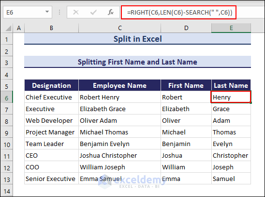

Here’s an alternative formula:

Select cell D6 and enter the below formula.

=LEFT(C6,FIND(" ",C6)-1)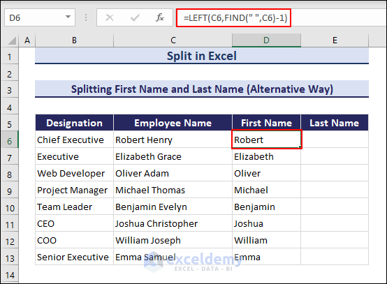

Use this formula in E6 and AutoFill to get the last names of the employees.

=RIGHT(C6,LEN(C6)-FIND(" ",C6))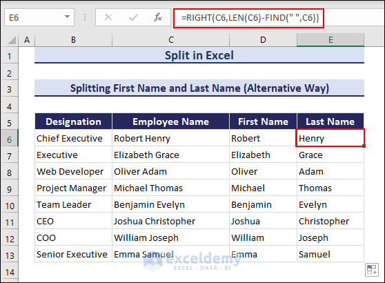

Method 2.2 – Splitting the First Name, Middle Name, and Last Name

The dataset contains the employee name “Robert Adam Henry” in cell C6. We need to split it into three columns.

Use the formula from the previous method to extract the first names.
Enter the below formula in cell E6 to get the middle name as output.

=IFERROR(MID(C6,SEARCH(" ",C6)+1,SEARCH(" ",C6,SEARCH(" ",C6)+1)-SEARCH(" ",C6)),"")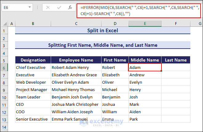

Enter the below formula in cell F6 to get the last name.

=IF(LEN(C6)-LEN(SUBSTITUTE(C6," ",""))=1,RIGHT(C6,LEN(C6)-SEARCH(" ",C6)),RIGHT(C6,LEN(C6)-SEARCH(" ",C6,SEARCH(" ",C6)+1)))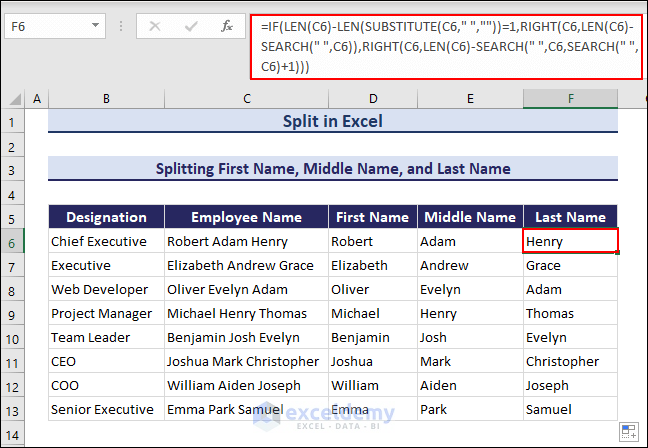

Part 3 – Applying the TEXTSPLIT Function to Split Cells Across Columns and Rows

The TEXTSPLIT function splits text strings through column and row delimiters. It returns multiple separate values as an array.

Method 3.1 – Split Cells Horizontally Across Columns

Apply the below formula to cell D6 and get both first and last names as output in individual cells.

=TEXTSPLIT(C6," ")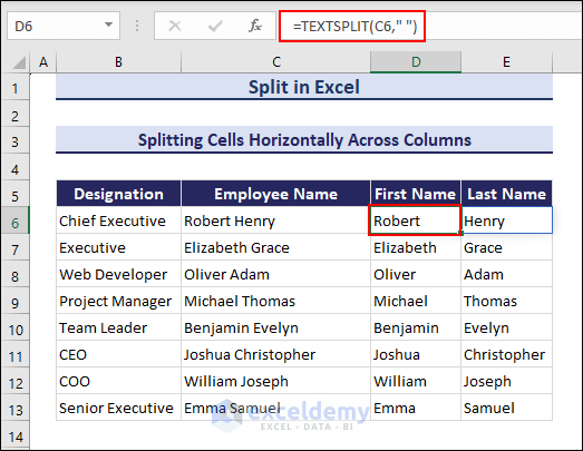

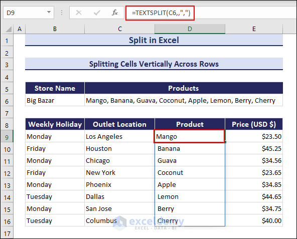
Method 3.2 – Split Cells Vertically Across Rows

Use the following formula to cell D9 to get the split data from cell C6.

=TEXTSPLIT(C6,,",")

The second argument is empty to force the formula to split vertically rather than horizontally. The output is Mango, Banana, Guava, Coconut, Apple, Lemon, Berry, and Cherry vertically. Some values will have spaces.

Note: The TEXTSPLIT function is only available for Microsoft 365 users. It is the inverse function of the TEXTJOIN function.

Part 4 – How to Separate Numbers from Text in Excel

The dataset contains an employee bio where the name, joining year, and experience are shown as a single cell, “Robert Henry, Joined in 2022, First Job”, so we will get the joining year – 2022.

Apply the below formula in cell D6.

=TEXTJOIN("",TRUE,IFERROR(MID(C6,ROW(INDIRECT("1:"&LEN(C6))),1)*1,""))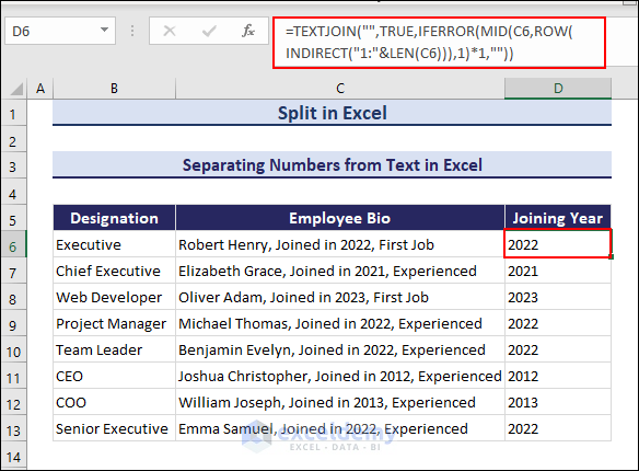

Part 5 – How to Split Merged Cells into Multiple Columns

The employee bio is merged into columns C and D. Here the Employee Bio is “Robert Henry, Joined in 2022”. We have a comma delimiter.

Apply the formula in cell E6 and split the merged cells into multiple columns.

=TEXTSPLIT(C6,",")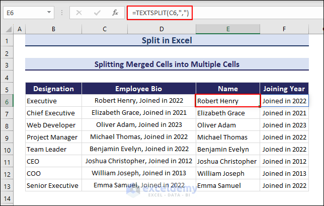

Part 6 – How to Split Text while Ignoring Missing Values

The fourth argument of the TEXTSPLIT function is ignore_empty. This argument is set to FALSE by default. So, this function doesn’t ignore the missing value by default and returns a blank cell for each missing value. If we set the ignore_empty argument to TRUE it will ignore the missing values.

Apply the formula in cell D6 and split cells while ignoring blank cells.

=TEXTSPLIT(C6,",",,TRUE)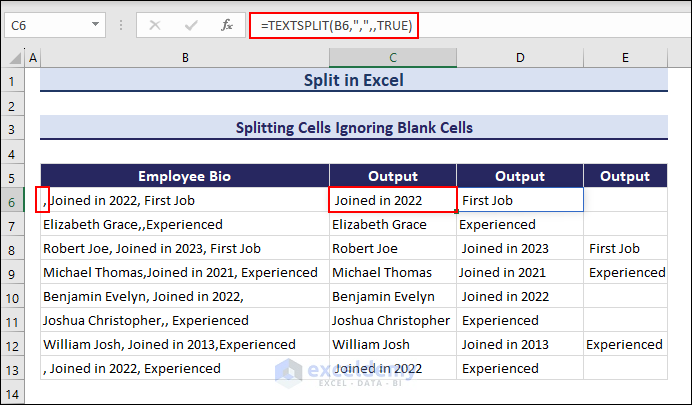

Part 7 – How to Split Columns Using Power Query

Select cell range C6:C13, go to the Data tab, and select Get Data from the toolbar.

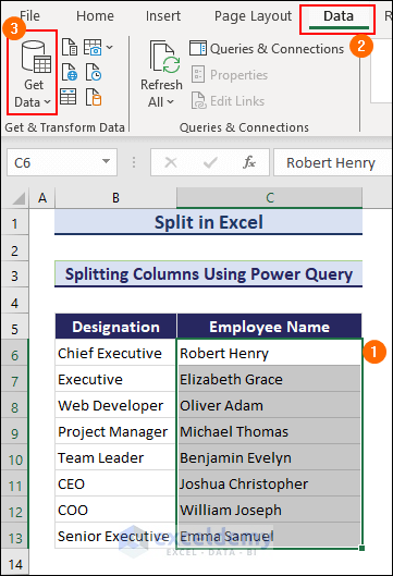
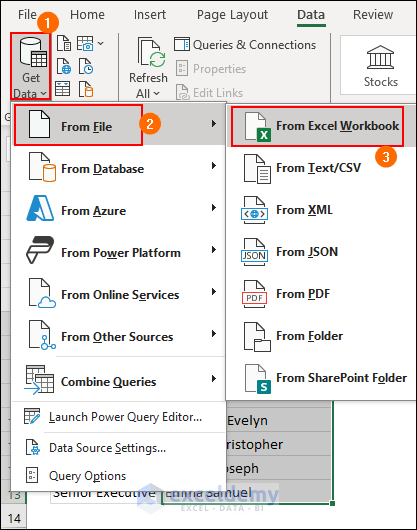
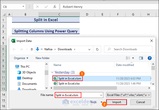
Select Get Data, choose From File, and select From Excel Workbook to get the Import Data dialog box.

Select the Excel file from the Import Data dialog box and click Import to open the Navigator window.

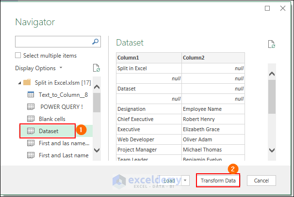
Select the sheet from the Navigator tab and hit Transform Data to transform the data.

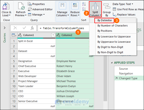
Select the column to split and go to Split Column.
Select By Delimiter.

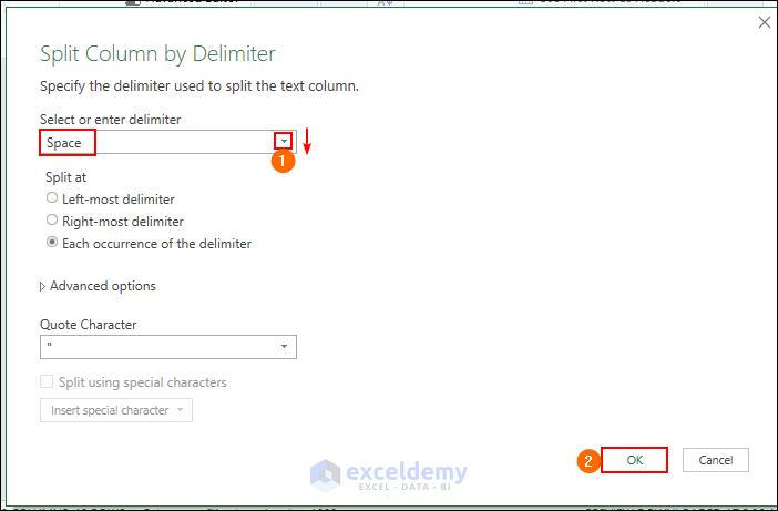
Select Space (or your delimiter) from the select or enter delimiter option and click OK to split the columns.

End the process by clicking the Close & Load option.

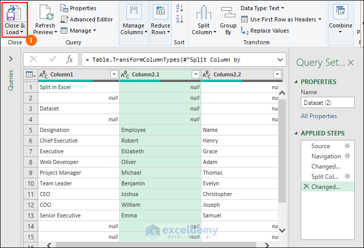
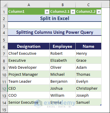
Here, the full name is split into columns B and C.

Part 8 – How to Apply VBA Macro to Split Cells

Go to the Developer tab and select Visual Basic, and a Visual Basic window will open to enter the code.
Go to Insert and select Module to get a blank module to write the code.
Insert the following code.

Sub SplitText()
Set ws = ThisWorkbook.Sheets("VBA")
lastRow = ws.Cells(ws.Rows.Count, "C").End(xlUp).Row
For Each cell In ws.Range("C6:C" & lastRow)
splitValues = Split(cell.Value, " ")
For i = 0 To UBound(splitValues)
If ws.Columns.Count < cell.Column + i + 1 Then
ws.Columns(cell.Column + i + 1).Insert
End If
cell.Offset(0, i + 1).Value = splitValues(i)
Next i
Next cell
End Sub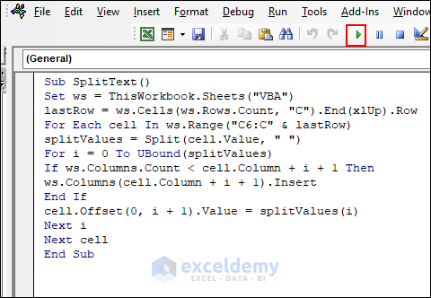

Note: We added a button to apply the code with a simple click. Go to Developer >> Insert >> Button (icon)

Run the code.

Download the Practice Workbook

Split in Excel.xlsm

Split in Excel: Knowledge Hub

<< Go Back to Learn Excel

Get FREE Advanced Excel Exercises with Solutions!