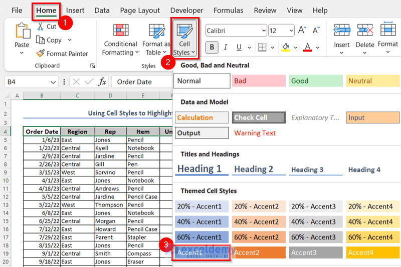
Method 1 – Using Cell Styles to Highlight Cells
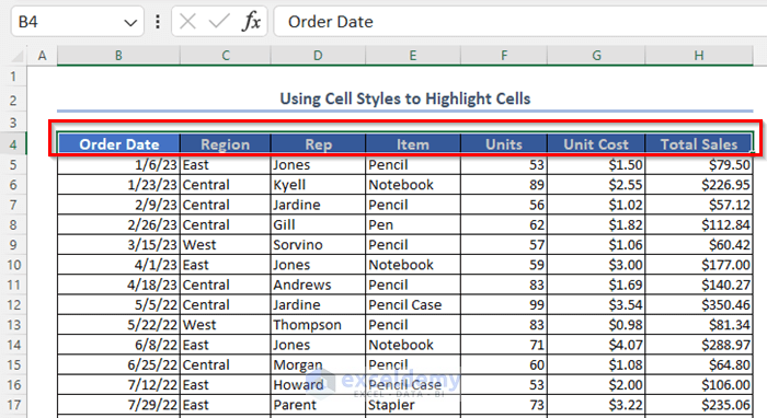
- Select cells >> go to the Home tab >> Styles >> select Cell Styles >> choose a style. Here, Accent1.
This is the output.
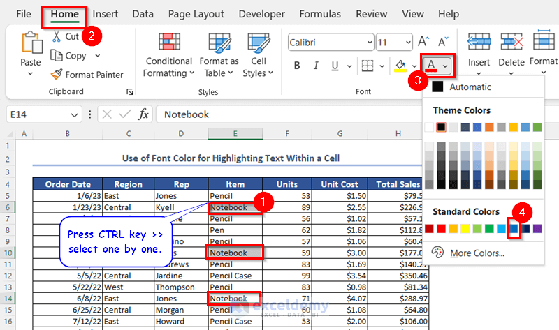
Method 2 – Use the Font Color to Highlight a Text Within a Cell
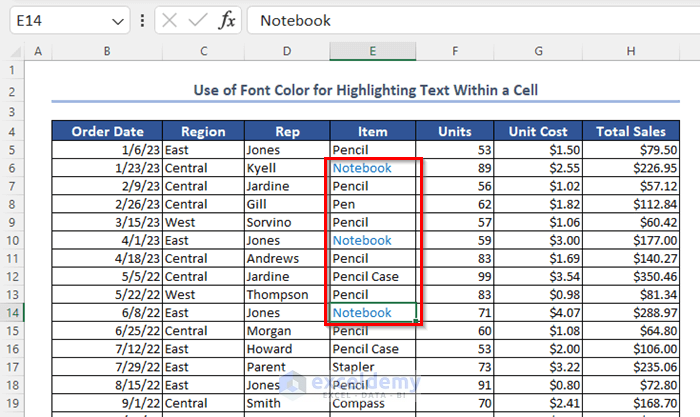
- Press CTRL >> select the target cells one by one >> go to the Home tab >> Font >> set a color.
This is the output.
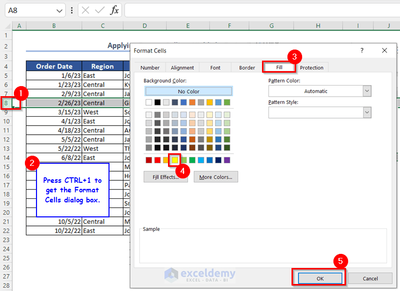
Method 3 – Applying Format Cells to Highlight an Entire Row
- Click the row index >> press CTRL+1 to display the Format Cells dialog box.
- Go to Fill >> choose a background color >> click OK.
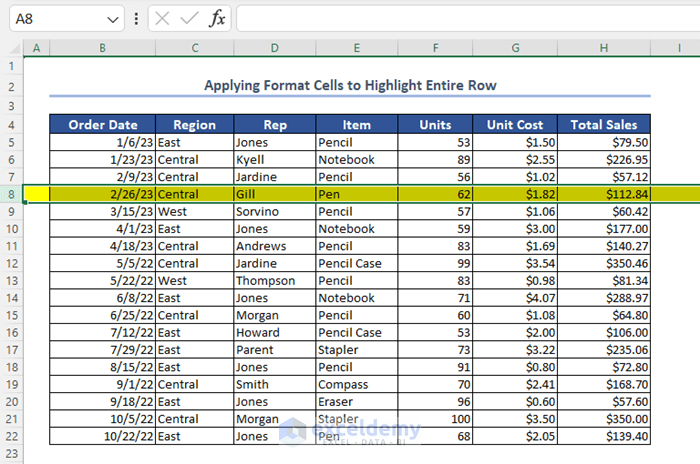
This is the output.
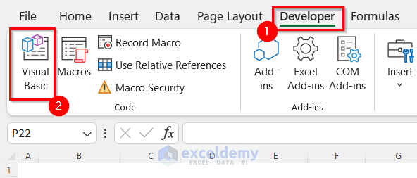
Method 4 – Using a VBA Code to Highlight Alternate Rows in Excel
- Go to the Developer tab >> Visual Basic.
- Open the VB Editor.
- In Insert >> choose Module >> enter the following code in Module1.
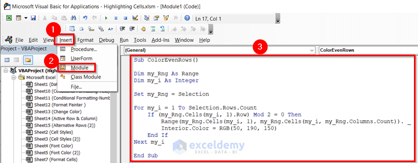
Sub ColorEvenRows()
Dim my_Rng As Range
Dim my_i As Integer
Set my_Rng = Selection
For my_i = 1 To Selection.Rows.Count
    If (my_Rng.Cells(my_i, 1).Row) Mod 2 = 0 Then
        Range(my_Rng.Cells(my_i, 1), my_Rng.Cells(my_i, my_Rng.Columns.Count)). _
        Interior.Color = RGB(50, 190, 150)
    End If
Next my_i
End Sub
Code Breakdown
- a sub-procedure is created: ColorEvenRows.
- my_Rng is declared as Range and my_i as Integer.
- The Selection property is used: the code will run in the selected cells.
- The For Next loop will go till the last row of the selected cells.
- The If End If statement will check whether the row number is even or odd.
- If the row number is even, the filled cells will be colored with the RGB color combination of 50,190 and 150.
- RGB is a function that defines color by combining red, green, and blue. The RGB function takes three arguments: the red value, the green value, and the blue value. Each of them is ranging from 0 to 255.
- Save the code and go back to the worksheet.
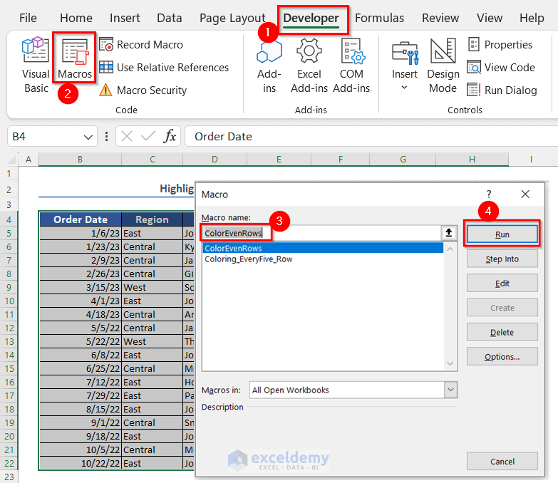
- Developer tab >> go to Macros >> in the Macro dialog box >> name the macro >> click Run.
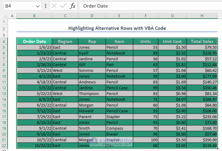
This is the output.
Method 5 – Using the Find and Replace Feature to Highlight Cells
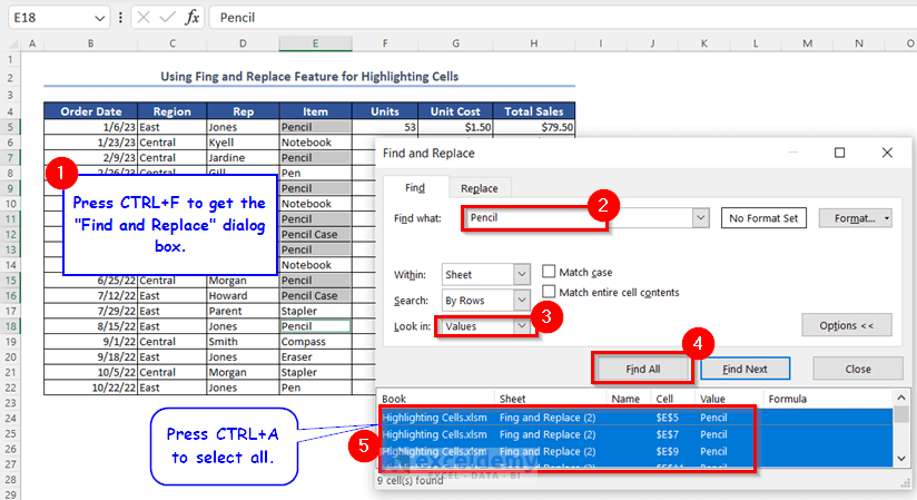
- Select the whole data >> press CTRL+F to display the Find and Replace dialog box.
- In the Find and Replace dialog box >> go to Find >> in Find what:, enter Pencil >> in Look in, select Values >> click Find All >> press CTRL+A to select the result.
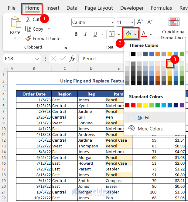
- In the Home tab >> go to Font >> Fill Color >> choose a color. Cells containing “Pencil” are highlighted.
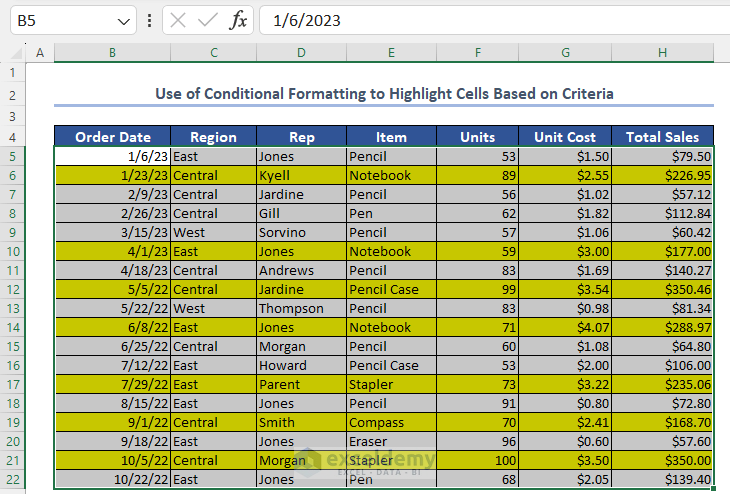
Method 6 – Use the Conditional Formatting to Highlight Cells Based on Criteria in Excel
6.1 Highlight Text Values that contain a feature
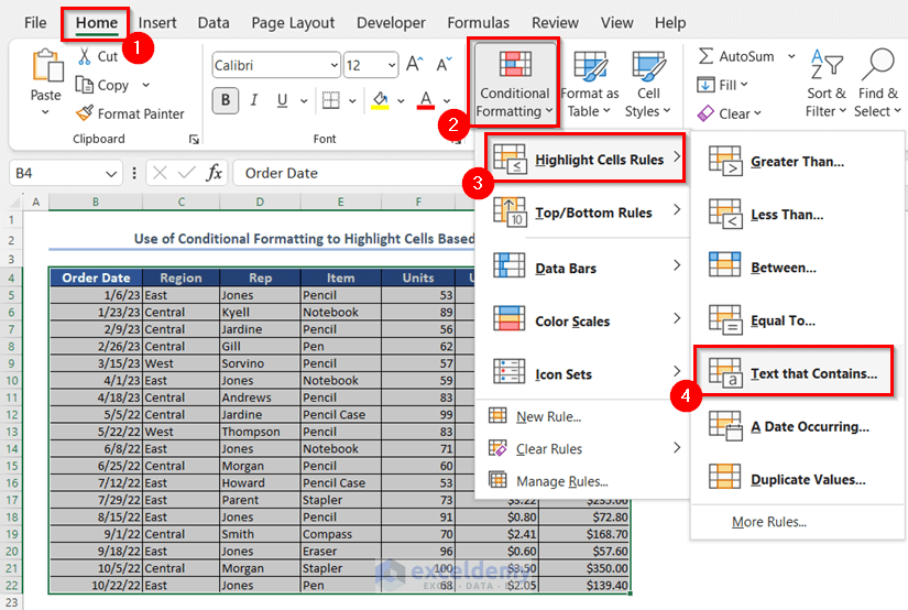
- Select the dataset >> in the Home tab >> go to Styles >> Conditional Formatting >> Highlight Cells Rules >> select Text that Contains.
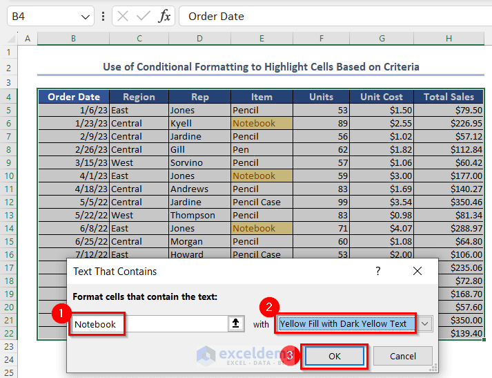
- In the dialog box, enter “Notebook” in Format cells that contain the text >> choose a color >> click OK.
- Cells containing “Notebook” are highlighted.
6.2 Using a New Rule to Highlight Cells Having Values That meet the Formula
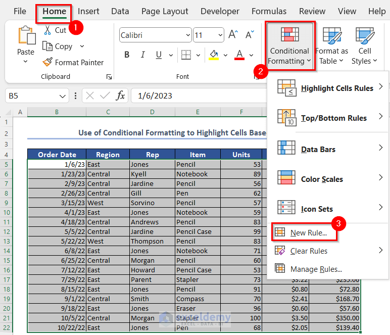
- Select the dataset (don’t select the headers) >> in the Home tab >> go to Styles >> Conditional Formatting >> select New Rule.
- In the New Formatting Rule dialog box >> select Use a formula to determine which cells to format >> go to Format values where this formula is true >> enter the formula >> click Format >> go to Fill >> set a color >> click OK to Format Cells >> click OK in New Formatting Rule.
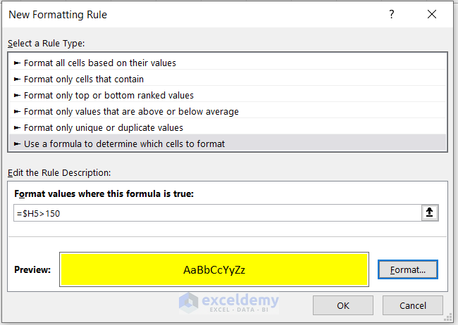
This is the output.
How to Use the Format Painter to Highlight Other Cells
- Select the cell >> in the Home tab >> go Clipboard >> double-click the Format Painter.
You will see a plus icon with the brush.
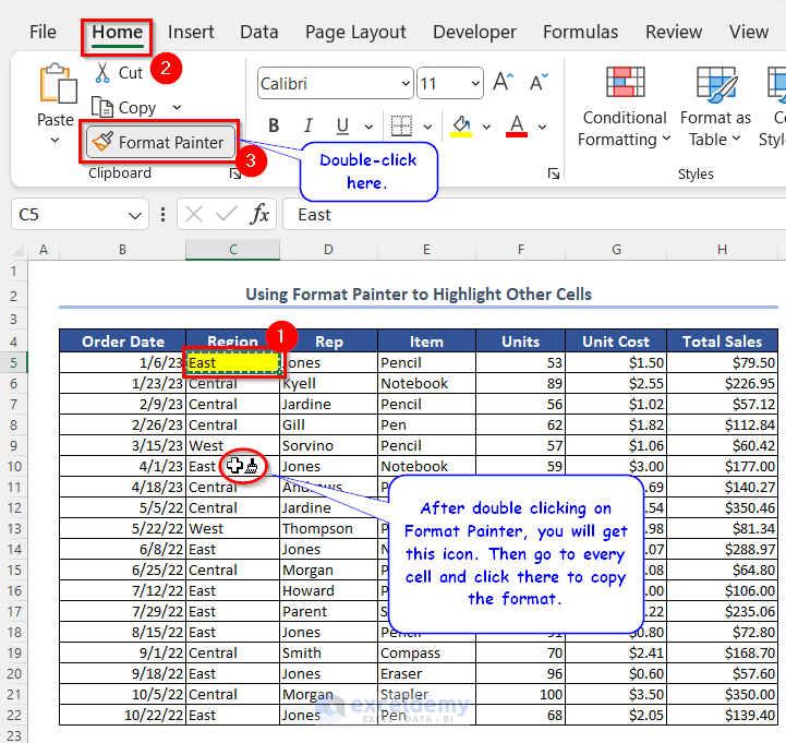
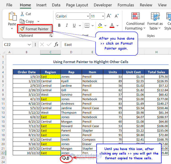
- Select cells and click the icon to copy the format.
- Click Format Painter again to stop copying the format.
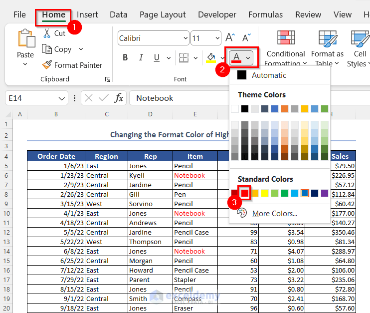
How to Change the Format Color of a Highlighted Text
- Select the cells you want to change.
- In the Home tab >> go to Font >> Font Color >> set a new color.
How to Highlight an Active Row and Column in Excel
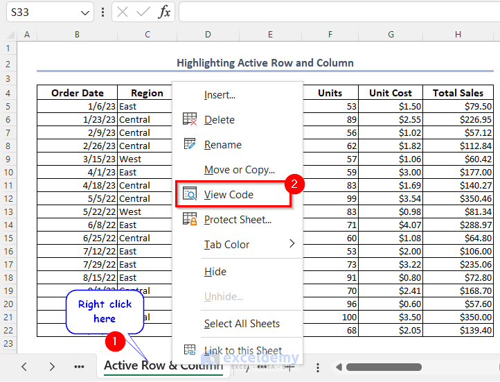
- Right-click the name of the sheet >>in the Context Menu Bar >> select View Code.
- Copy the code to the VB Editor.
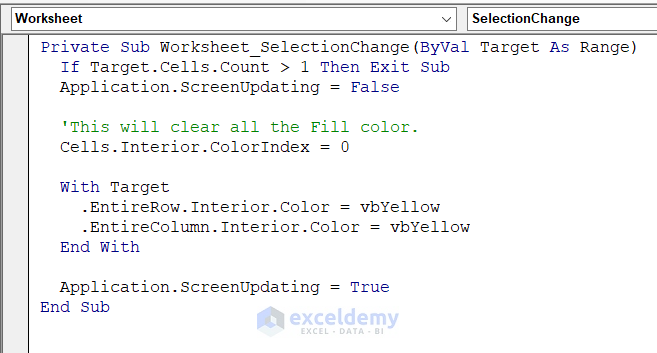
Private Sub Worksheet_SelectionChange(ByVal Target As Range)
  If Target.Cells.Count > 1 Then Exit Sub
  Application.ScreenUpdating = False
  'This will clear all the Fill color.
  Cells.Interior.ColorIndex = 0
  With Target
    .EntireRow.Interior.Color = vbYellow
    .EntireColumn.Interior.Color = vbYellow
  End With
  Application.ScreenUpdating = True
End Sub
Code Breakdown
- This code will work while you change the selection.
- Keeps the interior color of cells 0 to remove the previous color.
- For the active row/column, sets a new color.
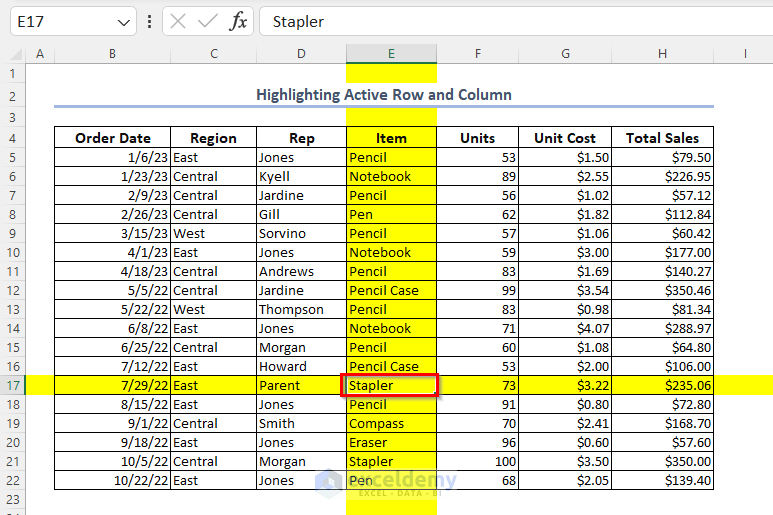
- Go to the selected sheet and click any cell to highlight the related row and column.
Frequently Asked Questions
1. What is the fastest way to highlight in Excel?
- Use SHIFT+Right/Left/Up/Down Arrow to select adjacent cells.
- Use CTRL key to select nonadjacent cells.
- Use CTRL+SHIFT+Right/Left/Up/Down Arrow to select all cells of the same row/column.
- In Fill Color >> set the color.
2. How do you highlight a column in Excel?
Click the column index number >> in Home tab >> Fill Color >> set the color.
3. How do I highlight part of text in an Excel cell?
Select that cell >> go to the Formula Bar >> select the text portion >> Font Color >> choose a color.
How to Highlight in Excel: Knowledge Hub
- Highlight Lowest Value in Excel
- Highlight Highest Value in Excel
- Highlight Text in Excel
- Highlight a Column
- Compare Two Excel Sheets and Highlight Differences
- Highlight Text in Text Box
- Highlight a Cell
Download Practice Workbook
Download the Excel file and practice.
<< Go Back to Learn Excel
Get FREE Advanced Excel Exercises with Solutions!

