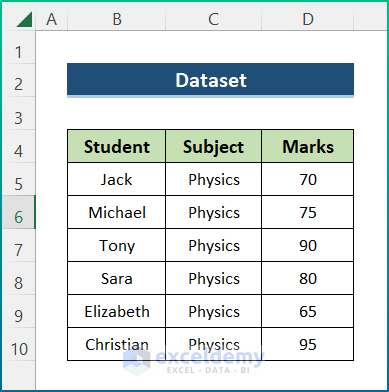
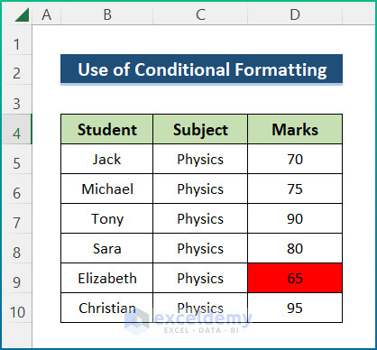
The following sample dataset includes 3 columns that consist of the Marks of some Physics Students.
Method 1 – Using the Sort & Filter Option to Highlight the Lowest Value
Steps:
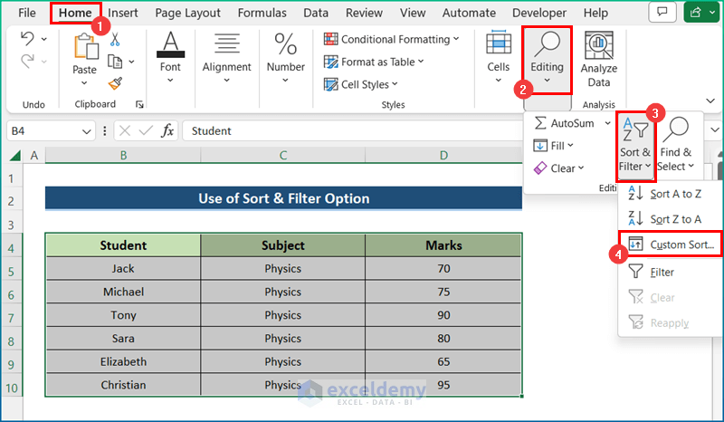
- Select the data range.
- Go to the Home tab>> Editing dropdown>> Sort & Filter dropdown>> Custom Sort option.
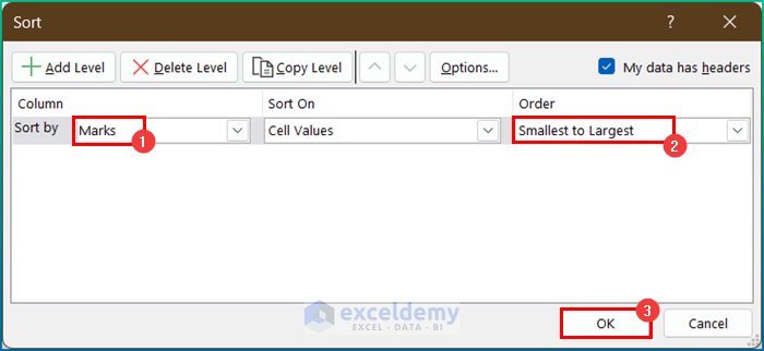
- The Sort Dialog Box will appear.
- Select the Marks on Sort by and choose Smallest to Largest for Order.
- Press OK.
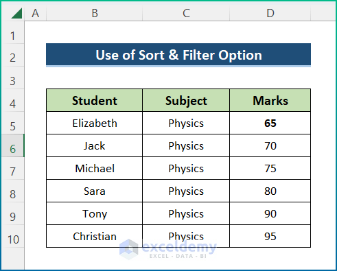
- You will get the values sorted in the smallest to largest order.
- Fill the D5 cell, which contains the lowest value after the sort operation, with any color if you wish to highlight the smallest value.
- You will get the highlighted lowest value.
Read More: How to Highlight Highest Value in Excel
Method 2 – Using the SMALL Function
Steps:
- Select Cell F5.
- Enter the following formula:
=SMALL(D5:D10,1)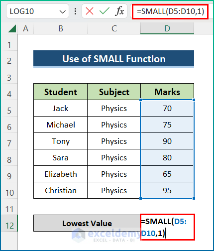
- Here, D5:D10 is an array, and 1 is the k-th value, which returns the k-th smallest value in a range.
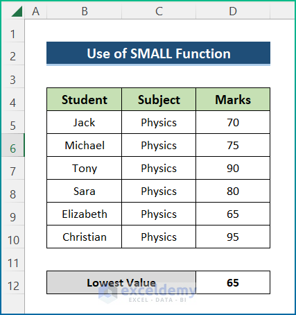
- You will get the lowest value among the marks of the students.
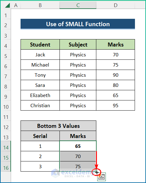
Method 3 – Finding Bottom 3 Values with SMALL Function
Steps:
- Select Cell G5.
- Enter the following formula:
=SMALL($D$5:$D$10,F6)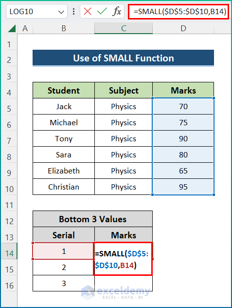
- Here, $D$5:$D$10 is an array, and F6 is the k-th value, which returns the k-th smallest value in a range.
- Press ENTER.
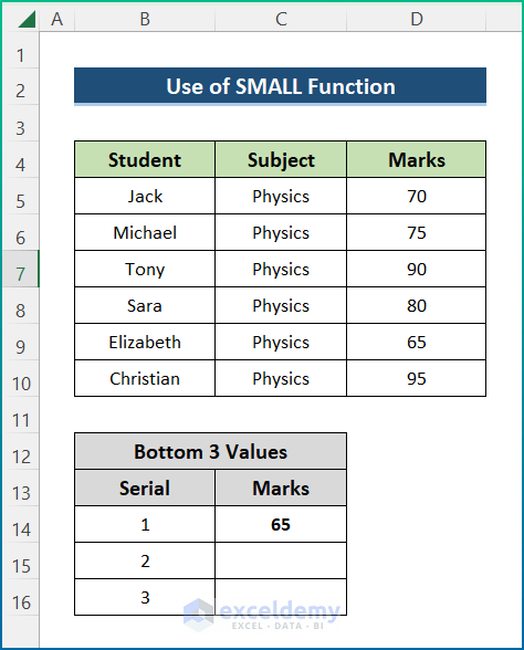
- Drag down the Fill Handle tool.
- You will get the lowest 3 values among the marks of the students.
Read More: How to Highlight a Column in Excel
Method 4 – Combining INDEX and MATCH Functions
Steps:
- Select Cell G5.
- Enter the following formula:
=INDEX(B5:B10,MATCH(SMALL($D$5:$D$10,F6),$D$5:$D$10,0))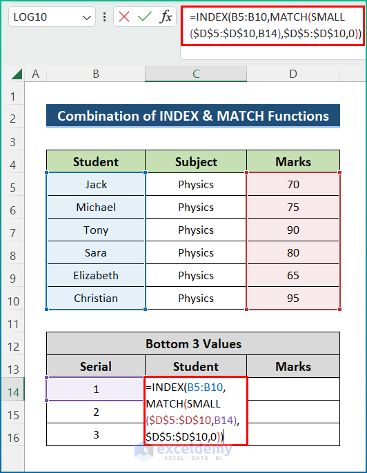
- Here, B5:B10 is the range of Student names,$D$5:$D$10 is the range of values, and F6 is the k-th value, which returns the k-th smallest value in a range. 0 is for an exact match.
- Press ENTER.
- Drag down the Fill Handle tool.
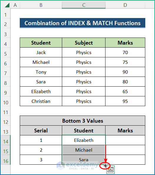
- You will get the names of the 3 students with the bottom 3 marks.
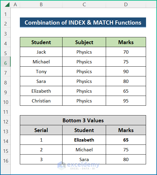
- Copy and Paste the marks according to the students in the Marks column.
- You will have the lowest 3 values here.
Method 5 – Combining SMALL and ROWS Functions to Sort Smallest to Largest Values
Steps:
- Select Cell E5.
- Enter the following formula:
=SMALL($D$5:$D$10,ROWS( D$5:D5))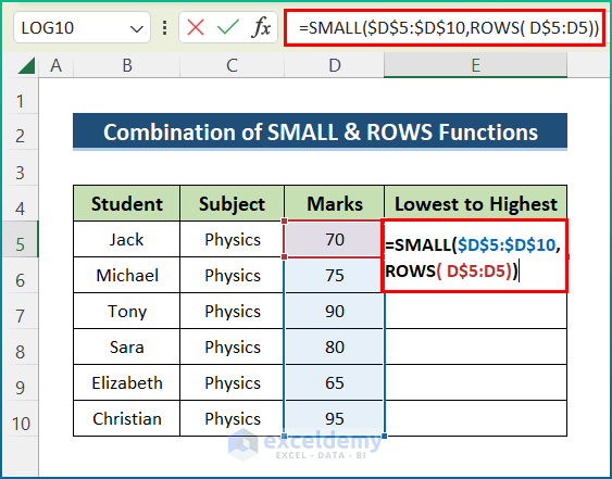
- Here, $D$5:$D$10 is an array, and ROWS( D$5:D5) will give the k-th value in each row.
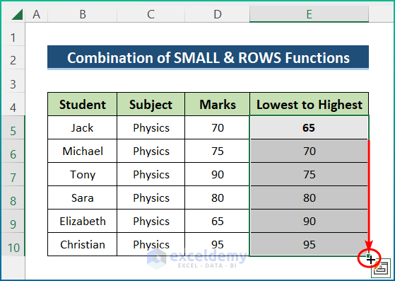
- Press ENTER.
- Drag down the Fill Handle tool.
- You will get the values in ascending order in the Lowest to Highest Marks column.
- Yu will get the highlighted lowest value.
Method 6 – Using Conditional Formatting
Steps:
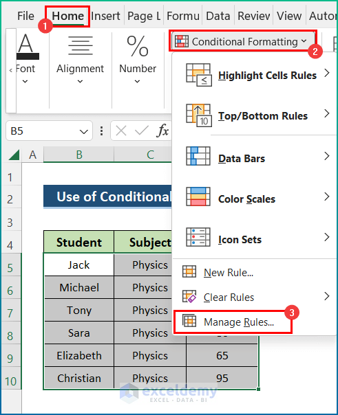
- Select the dataset, excluding the header.
- Go to the Home tab>> Conditional Formatting dropdown>> Manage Rules option.
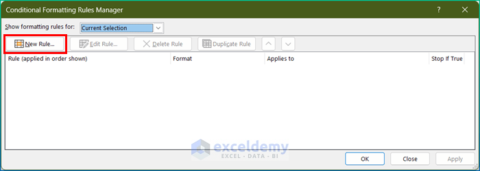
- The Conditional Formatting Rules Manager dialog box will appear.
- Select the New Rule option.
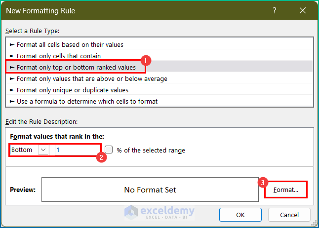
- The New Formatting Rule dialog box will appear.
- Select the Format only top or bottom ranked values option.
- Select Bottom and type 1 to get the lowest value only in the indicated area.
- Click on Format.
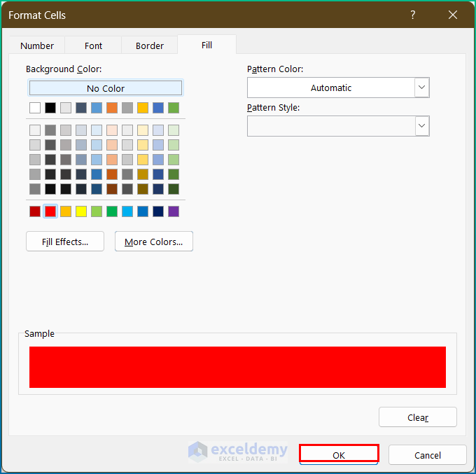
- The Format Cells wizard will pop up.
- Select any color of your wish.
- Press OK.
- Click OK.
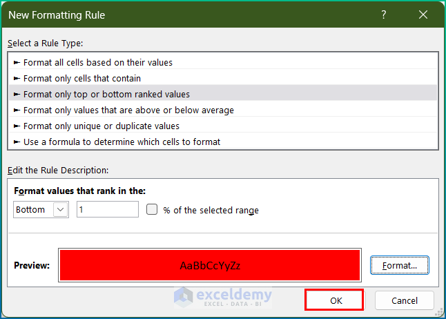
- Press OK.
- The lowest value in the Marks column will be highlighted.
Read More: How to Highlight Text in Excel
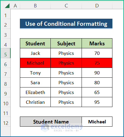
Method 7 – Highlighting the Smallest Value with Criteria
Steps:
- Select the dataset, excluding the header.
- Go to the Home Tab>> Conditional Formatting Dropdown>> New Rule Option.
- The New Formatting Rule dialog box will appear.
- Select the Use a formula to determine which cells to format option.
- Enter the following formula in the Format values where this formula is true:
=AND($B5=$F$6,$D5<=SMALL(IF($B$5:$B$12=$F$6,$D$5:$D$12),1))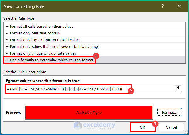
- Here, within the AND function, there are two criteria, and when these two are fulfilled, the cell will be highlighted.
- IF($B$5:$B$12=$F$6,$D$5:$D$12) will give an array including TRUE/FALSE when the value in F6 matches in the range $B$5:$B$12 or not and the corresponding value in the range $D$5:$D$12.
- Then this array goes to the SMALL function with a value of 1 for k and gives the lowest value.
- Follow the steps of Method 6.
- Afterward, you will get the lowest mark for Michael highlighted.
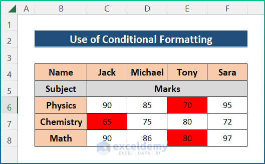
Method 8 – Highlighting the Lowest Value in Each Row
Steps:
- Follow Step-01 of Method-7.
- Enter the following formula:
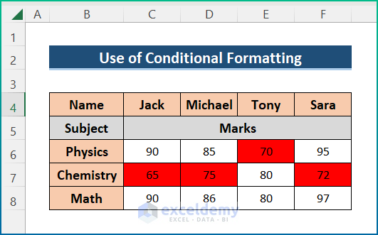
=C6=MIN($C6:$F6)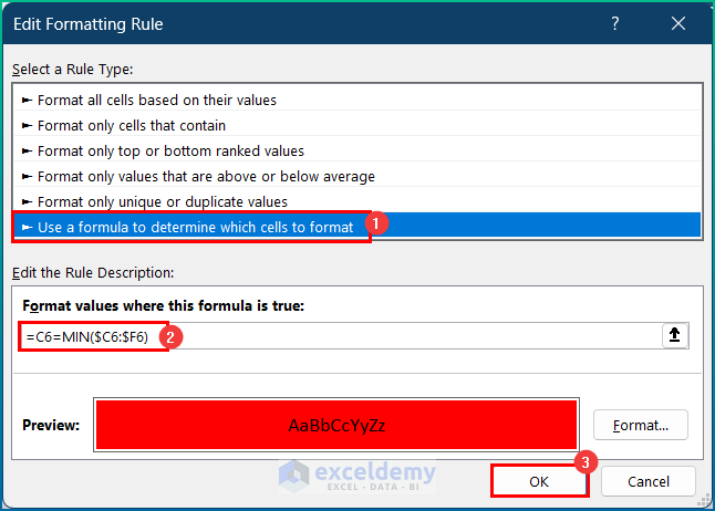
- Here, the MIN function will return the smallest value in each row.
- You will get the lowest values in each row.
Method 9 – Highlighting the Lowest Value in Each Column
Steps:
- Follow Step-01 of Method-7.
- Enter the following formula:.
=C6=MIN(C$6:C$8)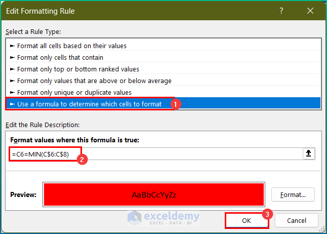
- Here, the MIN function will return the smallest value in each column.
- You will get the highlighted lowest values in each column.
Method 10 – Using SMALL Function for Dates
Steps:
- Select Cell E5.
- Enter the following formula: Here, C5:C9 is the range of dates.
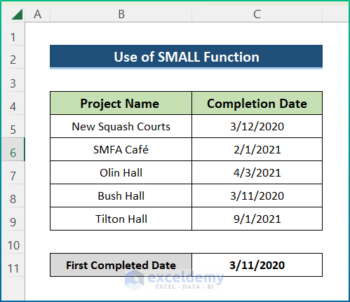
=SMALL(C5:C9,1)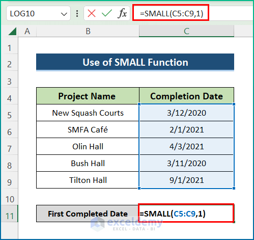
- Press ENTER.
- You will get the date of the first completed project.
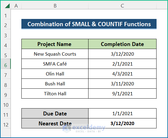
Method 11 – Finding the Previous Date Closest to a Specified Date
Steps:
- Select Cell E5.
- Enter the following formula:
=SMALL($C$5:$C$9,COUNTIF($C$5:$C$9,"<"&$E$4))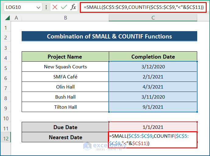
- Here, $C$5:$C$9 is the range of dates and
COUNTIF($C$5:$C$9,"<"&$E$4)will provide the value for k. - You will get the date before the due date.
Download the Practice Workbook
You can download the following workbook to practice.
Related Articles
- How to Compare Two Excel Sheets and Highlight Differences
- How to Highlight Text in Text Box in Excel
<< Go Back to Highlight in Excel | Learn Excel
Get FREE Advanced Excel Exercises with Solutions!
