How to Compare Two Excel Sheets and Highlight Differences: 7 Methods

Method 1 – Using the View Side by Side Option to Compare Two Excel Sheets from Different Files and Highlight the Differences

Steps:
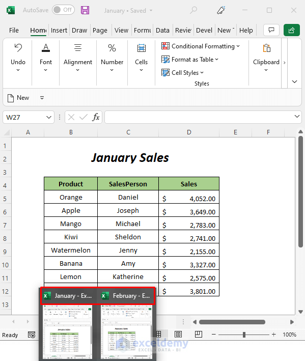
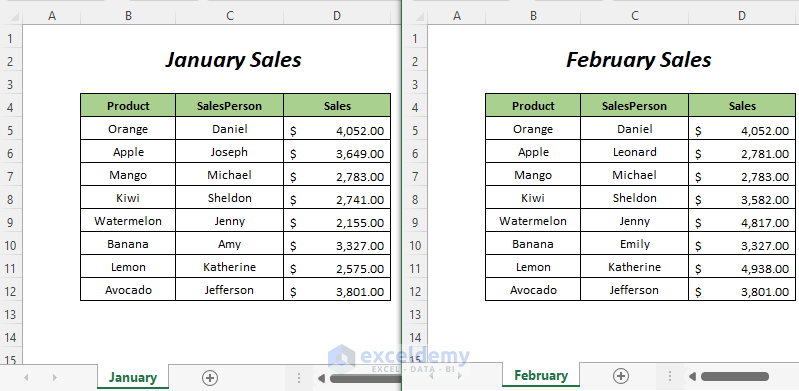
➤ Open the two workbooks simultaneously.

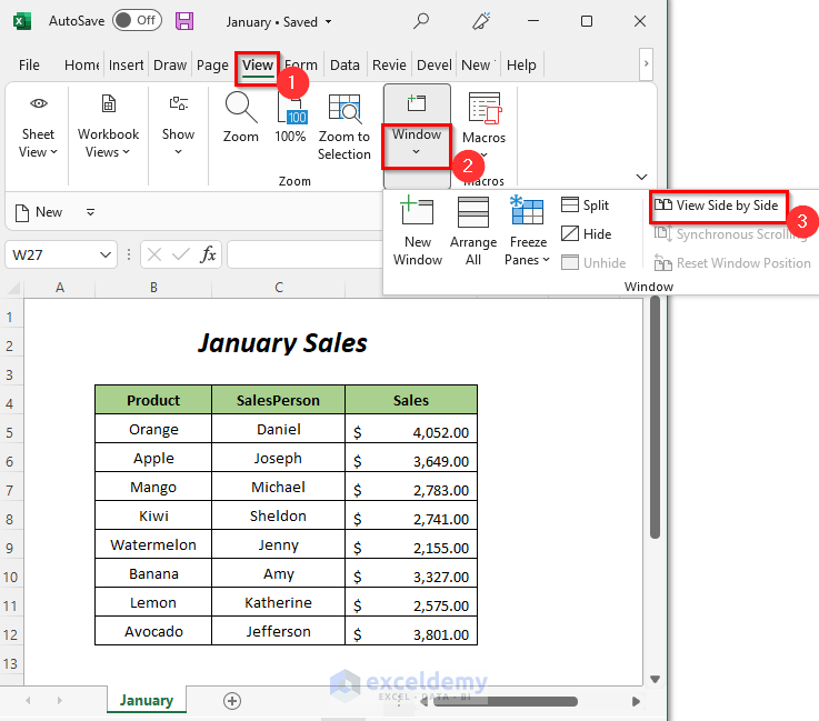
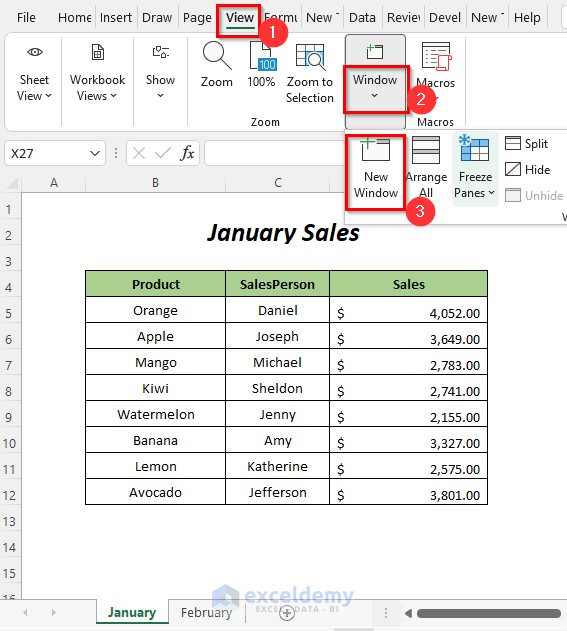
➤ Go to View Tab >> Window Dropdown >> View Side by Side Option

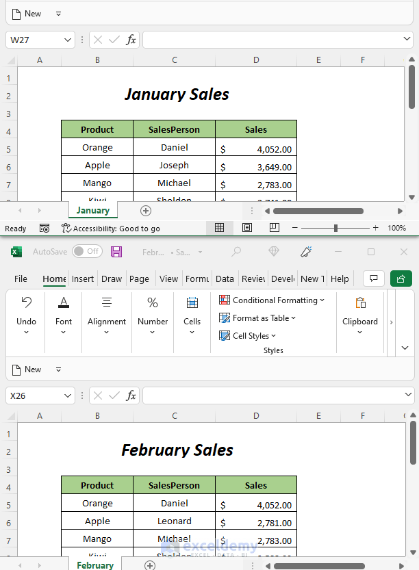
You will be able to view the two sheets at a time but they are aligned horizontally so we will change their alignment now.

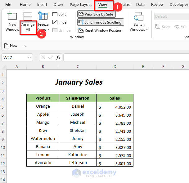
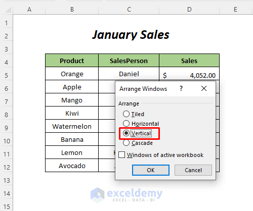
➤ Go to View Tab >> Window Group >> Arrange All Option.

The Arrange Windows will open up.
➤ Select the Vertical option and press OK.

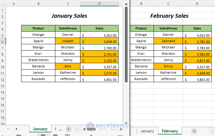
You can monitor the two sheets simultaneously, as shown below.

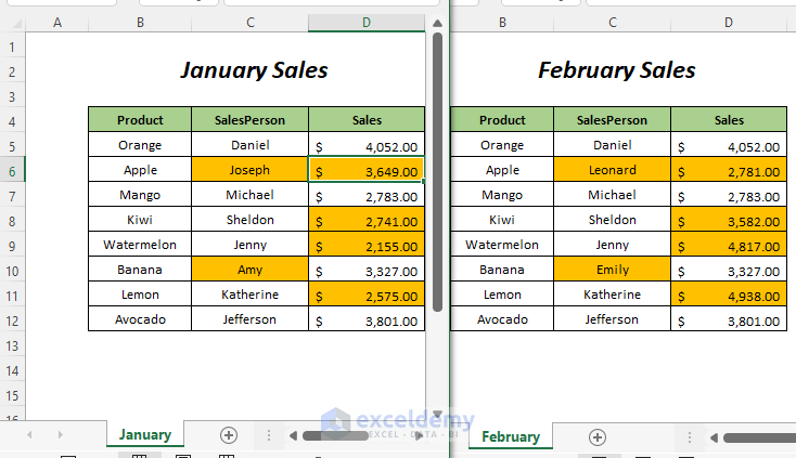
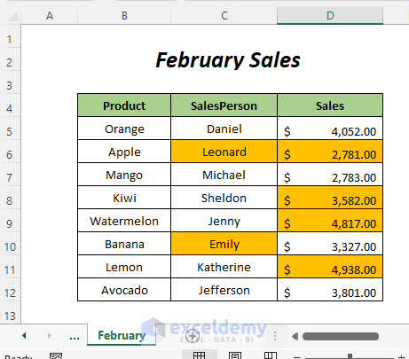
Select the cells of the SalesPerson column that have different names and change their background color.

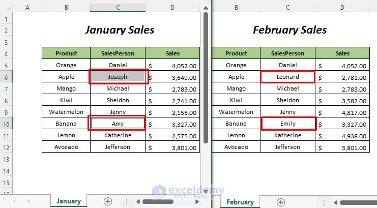
Get the highlighted cells that show the different names of the salespersons.

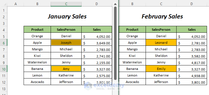
Select the cells of the Sales column that have different values and change their background color.

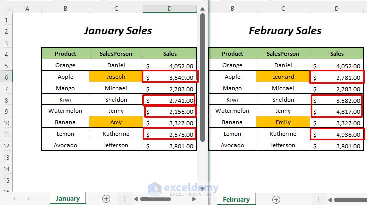
Get the highlighted cells having different values in the two sheets.

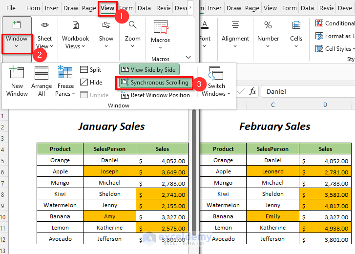
One thing to mention is that if you have a large dataset and you want to scroll through the values of these sheets simultaneously then you have to follow this way.
➤ Go to View Tab >> Window Group >> Synchronous Scrolling Option.

Method 2 – Utilizing Spreadsheet Compare Tool for Comparing Two Excel Sheets

Steps:
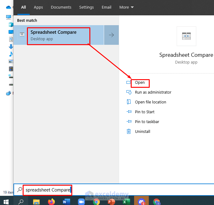
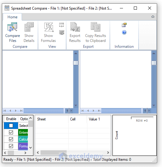
➤ Go to the Start screen, search for the Spreadsheet Compare app, and open it.

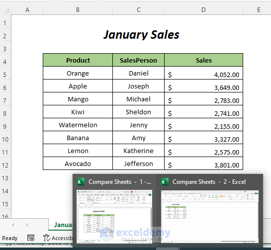
A new window Spreadsheet Compare will open up.

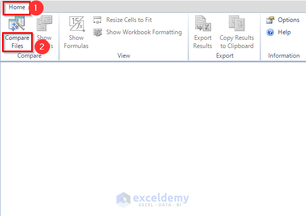
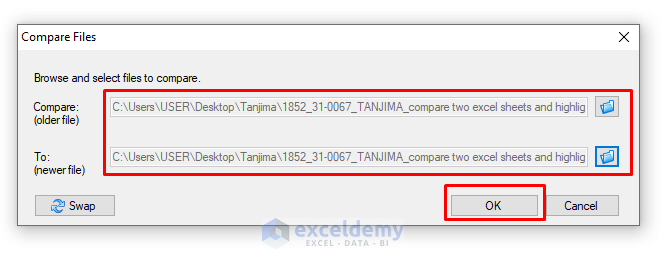
➤ Go to Home Tab >> Compare Files Option.

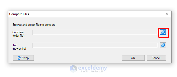
The Compare Files wizard will open up, and here select the indicated sign beside the Compare box to browse the location of the January file.

We have browsed the location of our January workbook.

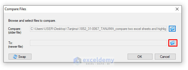
Choose the path of the file February workbook in the To box and press OK.

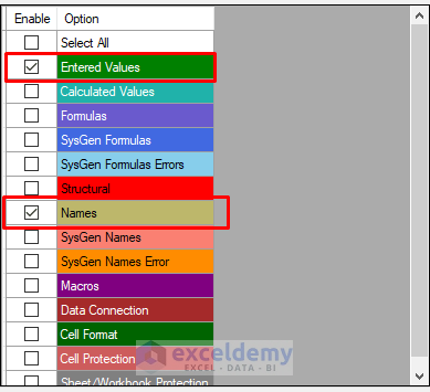
Select the options (based on which you want to compare the values of the workbooks) from the left pane. We selected the Entered Values and Names option.

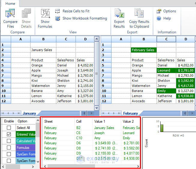
Get the highlighted values that show the differences between the two sheets, and here you can see the two sheets side by side that you are comparing. You are getting the description that indicates the different cells and values.

Note:
The Spreadsheet Compare option works for only Office Professional Plus 2013, Office Professional Plus 2016, Office Professional Plus 2019, and Microsoft 365 Apps.

Method 3 – Using the Compare and Merge Workbook Option

Step-01:
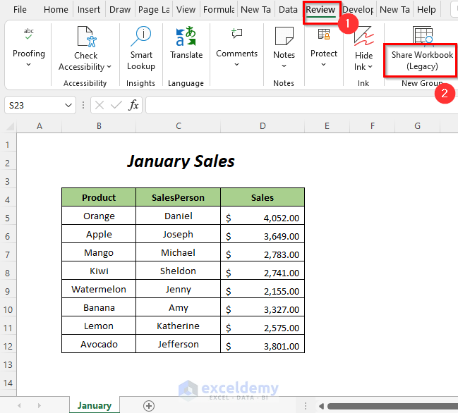
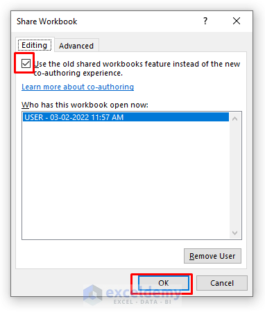
To enable the Compare and Merge Workbooks option, you have to follow this extra step.
➤ Go to Review Tab >> Share Workbook (Legacy) Option.

Then, the Share Workbook wizard will open up.
➤ Select the option “Use the old shared workbooks feature instead of the new co-authoring experience” and press OK.

Step-02:
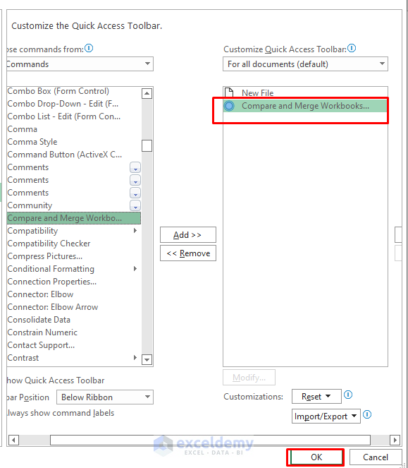
Add the Compare and Merge Workbooks option to the Quick Access Toolbar.
Go to the File Tab.

➤ Select Options.

The Excel Options wizard will open up, and here select the Quick Access Toolbar option.
➤ Select the options serially, All Commands → Compare and Merge Workbooks → Add.

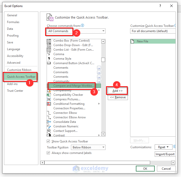
The Compare and Merge Workbooks option will be added to the toolbar, and press OK.

Step-03:
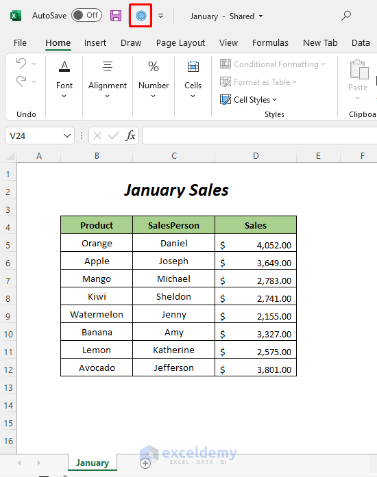
➤ Go to your main workbook January and select the Compare and Merge Workbooks option from the toolbar.

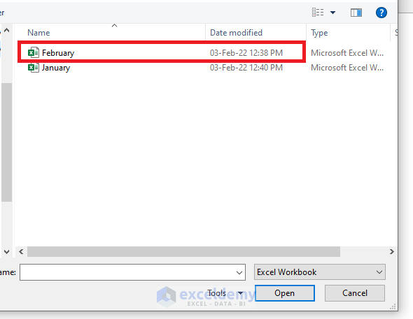
From the dialog box select the copy of your January file, which is February, and press OK.

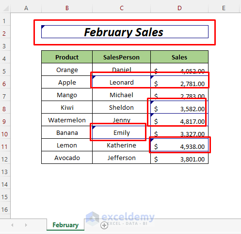
The changes we have made in the February workbook will appear in this workbook and those cells will be highlighted.

Method 4 – Applying the View Side by Side Option to Compare Two Excel Sheets and Highlight Differences from the Same File

Steps:
➤ Go to View Tab >> Window Group >> New Window option.

A new workbook will open up which is basically the same workbook that is opened right now and a slight change of name will be done automatically. See that the name of the opened workbook became Compare Sheets-1 and the name of the new workbook is Compare Sheets-2.

Follow the procedures of Method-1, and then you will be able to highlight the differences.

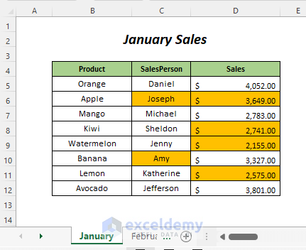
When you close any one of the workbooks, then the changes will appear in the two sheets of the main workbook like below.

Method 5 – Using Conditional Formatting to Compare Two Excel Sheets and Highlight Differences

Steps:
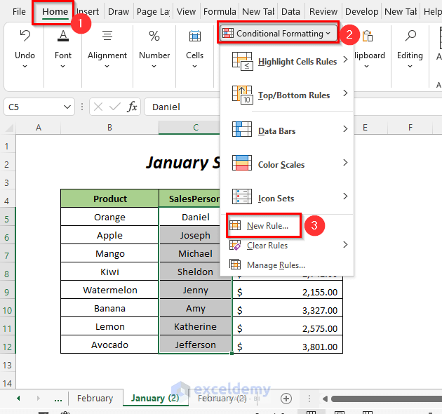
➤Select the data range on which you want to apply the Conditional Formatting
➤Go to Home Tab >> Conditional Formatting Dropdown >> New Rule Option.

The New Formatting Rule wizard will appear.
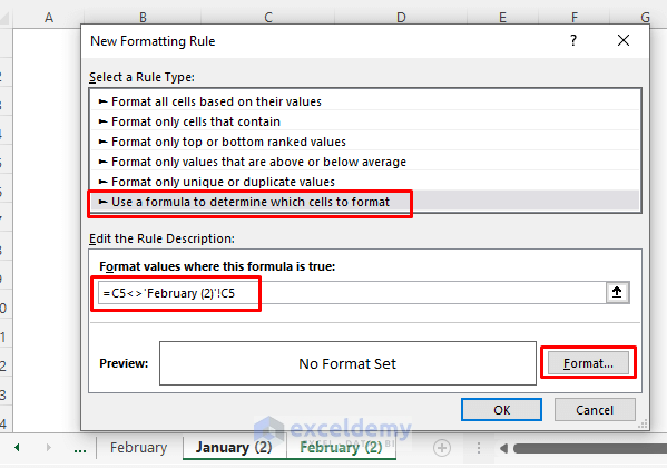
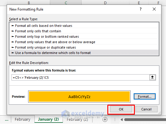
➤ Select Use a formula to determine which cells to format option and write the following formula in the Format values where this formula is true: box

=C5<>'February (2)'!C5

C5 is the first cell of the SalesPerson column, February (2) is the sheet name to which we want to compare and <> represents the Not Equal to operator.

➤ Click the Format option.

The Format Cells dialog box will open up.
➤ Select Fill Option.
➤ Choose any Background Color and click OK.

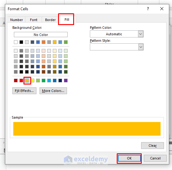
The Preview Option will be shown as below, and press OK.

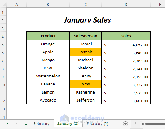
Get the highlighted cells in the SalesPerson column of the January (2) sheet.

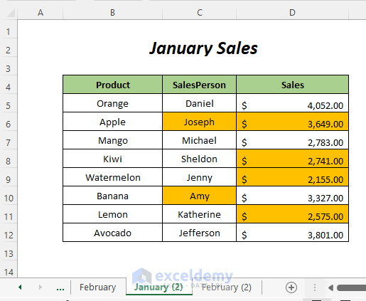
Highlight the different values of the Sales column.

Method 6 – Inserting a Formula to Combine the Differences in Another Sheet

Steps:
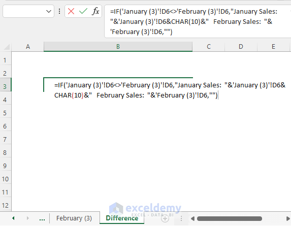
➤ Create a sheet named Difference and select a cell in this sheet.

➤ Write the following formula in the selected cell

=IF('January (3)'!D6<>'February (3)'!D6,"January Sales: "&'January (3)'!D6&CHAR(10)&" February Sales: "&'February (3)'!D6,"")

‘January (3)’! and ‘February (3)’! are the names of the sheets and when the values of the cells D6 will be not equal in these sheets then the corresponding values will be combined here otherwise IF will return a blank.

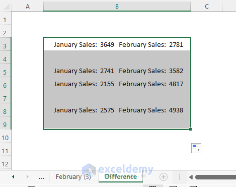
➤ Press ENTER and drag down the Fill Handle tool.

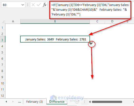
Get the different sales values for the January and February months.

Method 7 – Using a VBA Code to Compare Two Excel Sheets and Highlight Differences

Step-01:
➤ Go to Developer Tab >> Visual Basic Option.

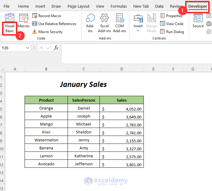
The Visual Basic Editor will open up.
➤ Go to Insert Tab >> Module Option

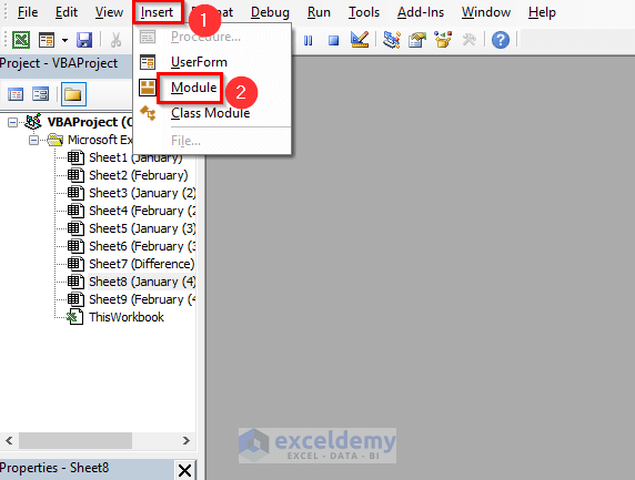
A Module will be created.

Step-02:
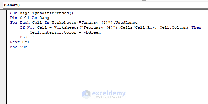
➤Write the following code

Sub highlightdifferences()

Dim Cell As Range

For Each Cell In Worksheets("January (4)").UsedRange
     If Not Cell = Worksheets("February (4)").Cells(Cell.Row, Cell.Column) Then
         Cell.Interior.Color = vbGreen
     End If
Next Cell

End Sub

We declared Cell as Range and used the VBA FOR Next loop for all of the used cells of the January (4) sheet, and the VBA IF statement will check the values of these cells with the values of the February (4). When the values are unequal, the color of those cells of the January (4) sheet will be changed to Green.

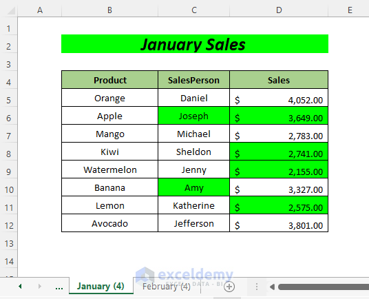
➤ Press F5.

Get the cells containing different values highlighted.

Download Practice Workbook

Compare Sheets.xlsm

<< Go Back to Highlight in Excel | Learn Excel

Get FREE Advanced Excel Exercises with Solutions!

Sub HighLight_Diff_in_same_Ws() Dim ws As Worksheet Dim cell_1 As Range, cell_2 As Range Set ws = ThisWorkbook.Sheets("Sheet1") For Each cell_1 In ws.Range("B5:D12") Set cell_2 = ws.Cells(cell_1.Row, cell_1.Column + 4) If Not (cell_1.Value = cell_2.Value) Then cell_1.Interior.Color = vbGreen cell_2.Interior.Color = vbGreen End If Next cell_1 End Sub

Sub HighlightChanges() Dim ws As Worksheet Dim rng As Range Dim cellAddresses As Variant Dim i As Integer ' Define the sheet and cell range to highlight Set ws = ThisWorkbook.Sheets("Sheet1") ' List of cell addresses cellAddresses = Array("A101", "B95", "B100", "B101", "C95", "C100", "C101", "D101") ' Loop through each address and highlight it For i = LBound(cellAddresses) To UBound(cellAddresses) ws.Range(cellAddresses(i)).Interior.Color = RGB(255, 255, 0) ' Highlight color Next i End Sub

Sub HighlightChangesFromFile() Dim ws As Worksheet Dim changesWs As Worksheet Dim rng As Range Dim cellAddresses As Variant Dim i As Integer Dim lastRow As Long ' Define the sheet to highlight and the sheet with cell addresses Set ws = ThisWorkbook.Sheets("Sheet1") Set changesWs = Workbooks("ChangesFile.xlsx").Sheets("Sheet1") ' Adjust workbook name ' Get the last row in column B for dynamic range lastRow = changesWs.Cells(changesWs.Rows.Count, "B").End(xlUp).Row ' Get the range of addresses from B3 to the last row Set rng = changesWs.Range("B3:B" & lastRow) ' Loop through each address and highlight it For Each cell In rng ws.Range(cell.Value).Interior.Color = RGB(255, 255, 0) ' Highlight color Next cell End Sub

8 Comments

Alejandro Oct 15, 2023 at 7:15 PM

Hello,

Thank you very much for this code.

Could you please help in comparing two tables in the same worksheet? For example, the ame second table starting at F4 for the example above.

Many thanks
- Reply
  Sourav Kundu Oct 16, 2023 at 11:32 AM
  Hello, ALEJANDRO
  Thank you for your comment. We have got an effective solution for your problem. We have taken 2 tables in the same worksheet as you can see from the following image:
  
  To compare between these 2 tables, you can use the following VBA code:
```
Sub HighLight_Diff_in_same_Ws()
    Dim ws As Worksheet
    Dim cell_1 As Range, cell_2 As Range
    Set ws = ThisWorkbook.Sheets("Sheet1")
    
    For Each cell_1 In ws.Range("B5:D12")
        Set cell_2 = ws.Cells(cell_1.Row, cell_1.Column + 4)
        If Not (cell_1.Value = cell_2.Value) Then
            cell_1.Interior.Color = vbGreen
            cell_2.Interior.Color = vbGreen
        End If
    Next cell_1
End Sub
```
  Note: You should modify the Worksheet Name, Range and Cells references according to your data table.
  
  When you run the VBA code, it will highlight the differences between the 2 tables in green color.
  
  I hope, this is the solution you were looking for. If you have further queries let us know in the comment section. We will solve them as soon as possible.
  
  Regards,
  Sourav Kundu.
  Exceldemy
Shan Sep 25, 2024 at 1:10 AM

Hello, I am using excel compare tool and it generates a new file with range(A101
B95
B100
B101
C95
C100
C101
D101
) of cells that have changed value.
I would like to take the range and highlight the corresponding excel file cells which has these changes.
- Reply
  Shamima Sultana Sep 25, 2024 at 10:11 AM
  Hello Shan,
  
  To highlight the range with changes, you’ll need to use VBA to highlight the changed cells in the original Excel file.
  
  If the compare tool generates a range like (A101, B95, etc.). You’ll need to copy this list.
  Open the workbook where changes occurred. Then, run the following VBA script to loop through the list and highlight the cells.
```
Sub HighlightChanges()
    Dim ws As Worksheet
    Dim rng As Range
    Dim cellAddresses As Variant
    Dim i As Integer
    
    ' Define the sheet and cell range to highlight
    Set ws = ThisWorkbook.Sheets("Sheet1")
    
    ' List of cell addresses
    cellAddresses = Array("A101", "B95", "B100", "B101", "C95", "C100", "C101", "D101")
    
    ' Loop through each address and highlight it
    For i = LBound(cellAddresses) To UBound(cellAddresses)
        ws.Range(cellAddresses(i)).Interior.Color = RGB(255, 255, 0) ' Highlight color
    Next i
End Sub
```
  It will highlight the specified cells with a yellow background.
  
  Regards
  ExcelDemy
  - Reply
    Shan Sep 26, 2024 at 12:26 AM
    
    This is working great, however the CellAddresses is different every time, could be 5/10/11 any number. Is there a way to feed the cell addresses from an excel file(Range always starts from cell B3) so it is dynamic?
    - Shamima Sultana Sep 26, 2024 at 12:09 PM
      
      Hello Shan,
      
      Glad to hear. To dynamically feed cell addresses from an Excel file (starting at cell B3), you can modify the VBA code to read the list directly from that file.
      
      Sub HighlightChangesFromFile() Dim ws As Worksheet Dim changesWs As Worksheet Dim rng As Range Dim cellAddresses As Variant Dim i As Integer Dim lastRow As Long ' Define the sheet to highlight and the sheet with cell addresses Set ws = ThisWorkbook.Sheets("Sheet1") Set changesWs = Workbooks("ChangesFile.xlsx").Sheets("Sheet1") ' Adjust workbook name ' Get the last row in column B for dynamic range lastRow = changesWs.Cells(changesWs.Rows.Count, "B").End(xlUp).Row ' Get the range of addresses from B3 to the last row Set rng = changesWs.Range("B3:B" & lastRow) ' Loop through each address and highlight it For Each cell In rng ws.Range(cell.Value).Interior.Color = RGB(255, 255, 0) ' Highlight color Next cell End Sub
      
      This will read the cell addresses from column B of the other file and highlights them in the current workbook. Remember to replace “ChangesFile.xlsx” with the actual name of your file.
      
      Regards
      ExcelDemy

Shan Sep 26, 2024 at 12:27 AM

Or even copy the CellAddresses from this other excel file to the workbook where changes occurred then VBA can use that to build the array then color?

Shamima Sultana Sep 26, 2024 at 12:09 PM

Hello Shan,

To dynamically feed cell addresses from an Excel file (starting at cell B3), you can modify the VBA code to read the list directly from that file.

This will read the cell addresses from column B of the other file and highlights them in the current workbook. Remember to replace “ChangesFile.xlsx” with the actual name of your file.

Regards
ExcelDemy