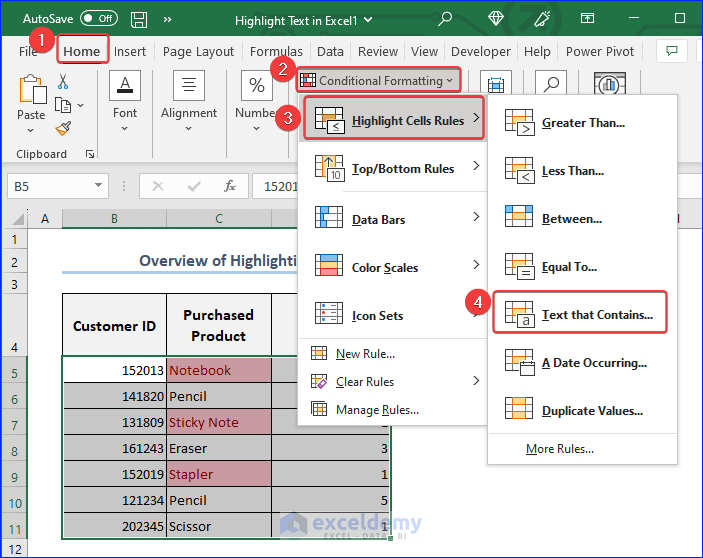
How to Highlight Text in Excel (7 Easy Ways)

Here’s an overview of where you can find the conditional highlight options in Excel.

Method 1 – Highlight Text in Excel Using the Font Color

Select the range of text you want to highlight.
Go to the Font group under the Home ribbon and click on Font Color.
Select any color from the Theme Colors group.

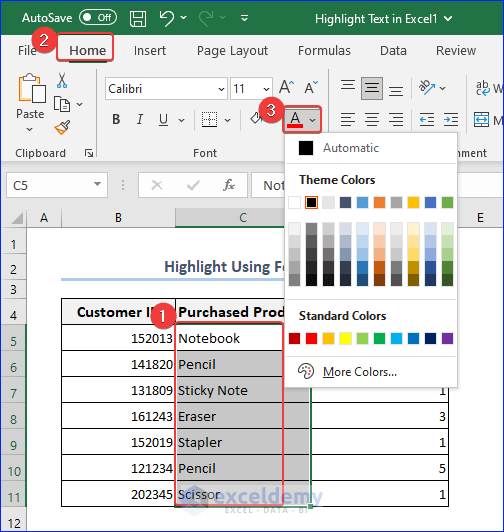
The output will look to the following image.

Method 2 – Using Excel Cell Styles to Highlight Text

Select the cells that you want to highlight.
Under the Home ribbon, select Cell Styles.
Choose any of the options.

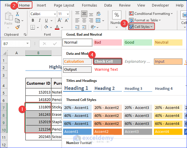
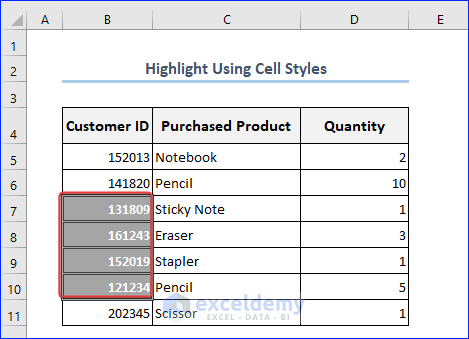
If you choose the option Check Cell, your output will look similar to the following image.

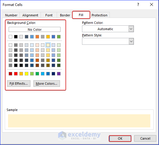
Method 3 – Highlight Specific Text Using Format Cells

Select the dataset.
Press Ctrl + 1 to open the Format Cells dialog box.

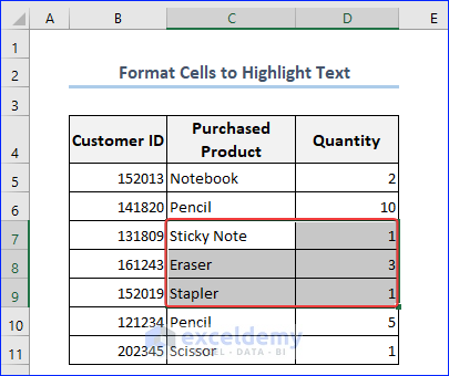
Change the options in the dialog box accordingly.

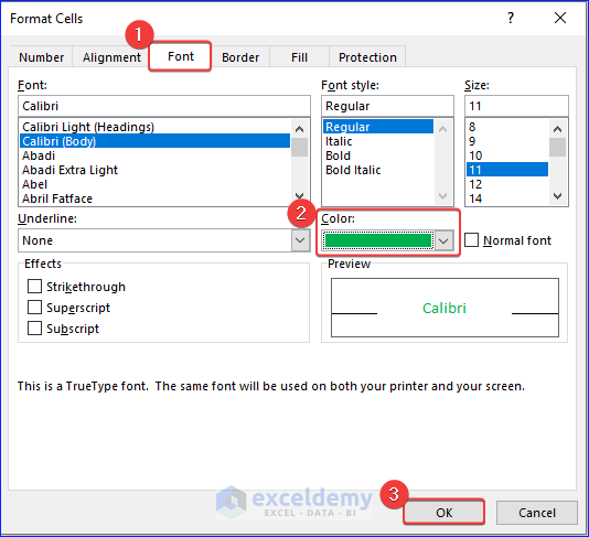
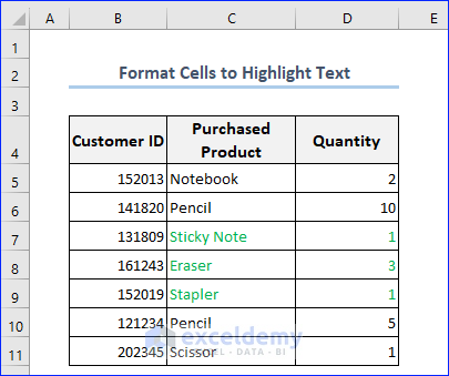
Here’s a sample result.

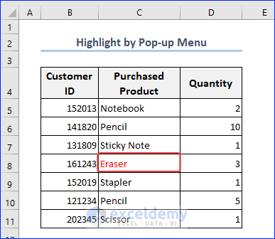
Method 4 – Using a Pop-up Menu to Highlight Text in Excel

Select the text in a certain cell. A pop-up menu would appear like the following image.
Click on the Font Color option and select any of the colors available to highlight the text.

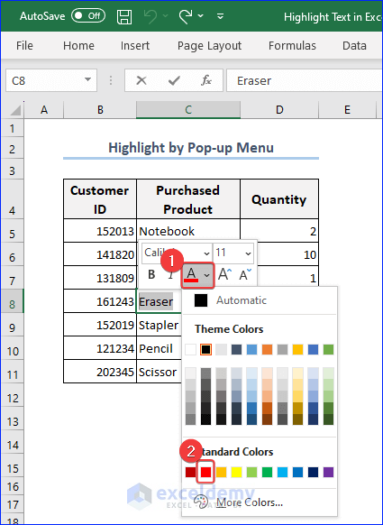
Here’s a sample result.

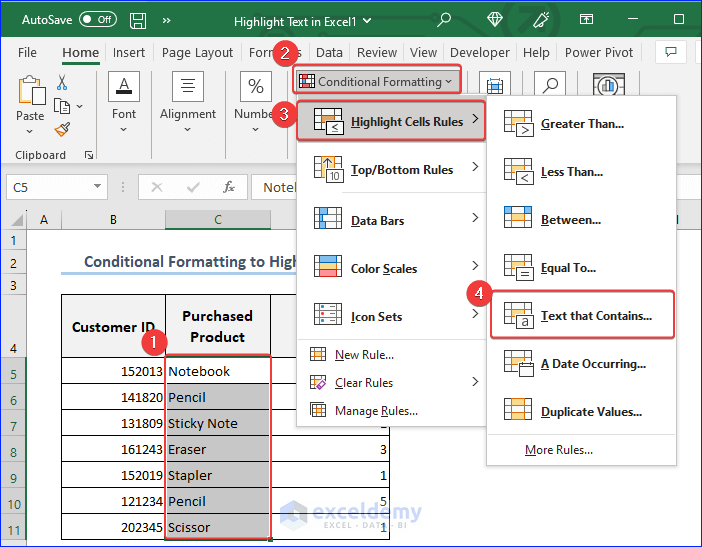
Method 5 – Highlight Text with Conditional Formatting

Select the range and then select Conditional Formatting under the Styles ribbon group from the Home.
We chose “Text that Contains” as a condition.

A dialog box appears. Provide the conditions based on which Excel will apply to format.

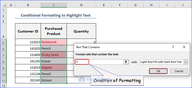
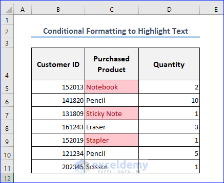
Your output will look like the following image.

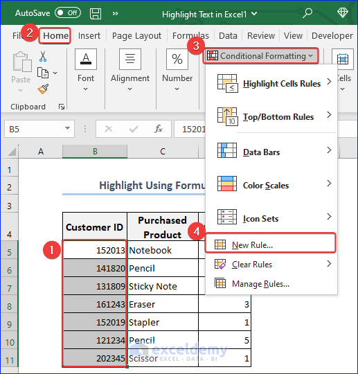
Method 6 – Highlight Text Using Excel Formula

Select the text where you will apply highlighting.
Go to Conditional Formatting and select New Rule.

Apply a formula in the box Format values where this formula is true:

=$B5>150000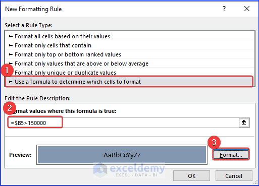

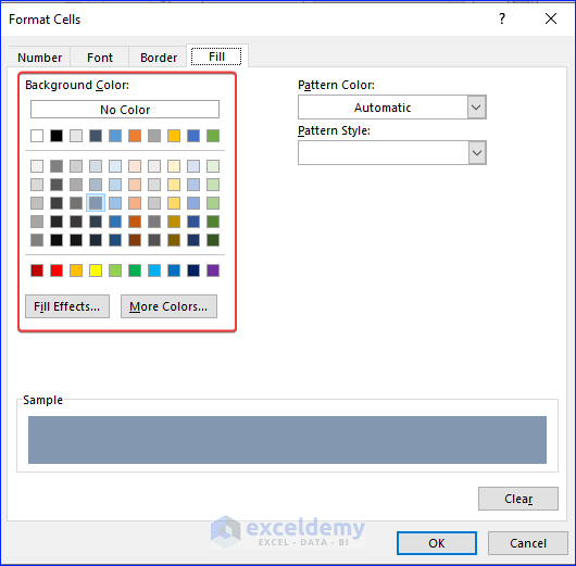
When you click on the Format… button, a dialog box will appear prompting you to choose a color for formatting.

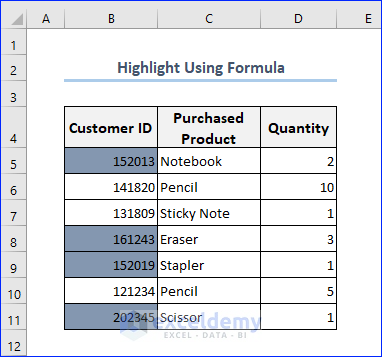
Here’s a sample result.

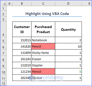
Method 7 – Applying Excel VBA Code to Highlight Text

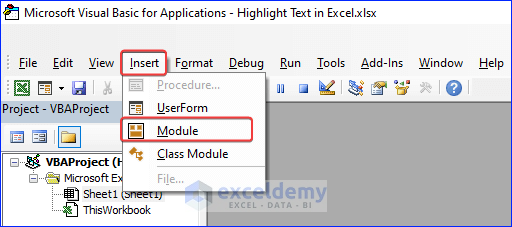
Press Alt + F11 to open the VBA Editor.
Under the Insert tab, click on Module.

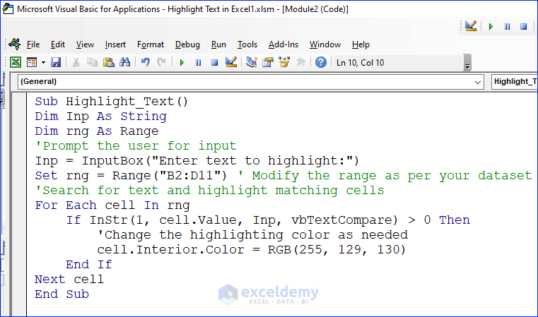
Copy the following VBA code.

Sub Highlight_Multiple()
Dim Input1 As Variant
Dim rng As Range
' Prompt the user for input
Input1 = Split(InputBox("Enter the words(separated by comma):"), ",")
' Set the range where you want to search for the text
Set rng = Range("B5:D11") ' Modify the range as per your dataset
' Clear any previous highlighting
rng.Interior.Pattern = xlNone
' Search for the words and highlight the matching cells
For Each word In Input1
    For Each cell In rng
        If InStr(1, cell.Value, Trim(word), vbTextCompare) > 0 Then
            'Change the highlighting color as needed
            cell.Interior.Color = RGB(255, 0, 0)
        End If
    Next cell
Next word
End Sub

Paste the code in the editor and save it.

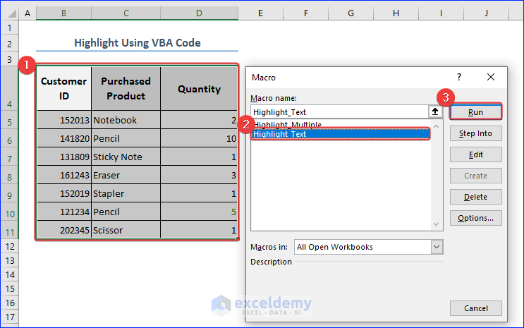
Go back to the Excel workbook and select the whole data table.
Press Alt + F8 to open the Macro window.
Select the Highlight_Text code and hit Run.

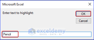
An input box will appear. Insert the text you want to highlight. We put “Pencil” in the box since we want to highlight it in the data table.

Your output will look like the following image.

How Does the Code Function?

Inp = InputBox(“Enter text to highlight:”)

Prompts the user to provide the text that the code will highlight. Assign the user’s input to a variable named “Inp”.

Set rng = Range(“B2:D11”)

Declares the variable “rng” to hold the range from B2 to D11 since our data is in this range.

For Each cell In rng

Loops through all the cells in the range “rng” and checks whether it meets certain criteria.

If InStr(1, cell.Value, Inp, vbTextCompare) > 0 Then

The VBA InStr function starts the comparison of text from the beginning of each “cell” in the “rng” variable. If it finds a match, then it will return a value greater than zero (the position of the starting substring in the first string). In that case, the condition becomes true, and the code is on the next line under the condition.

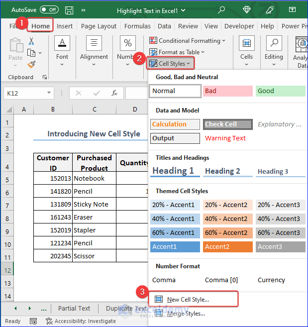
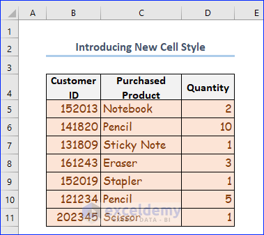
How to Create a Highlight Style in Excel

Select the Home tab and go to Cell Styles.
Under the Cell Styles group, click on New Styles.

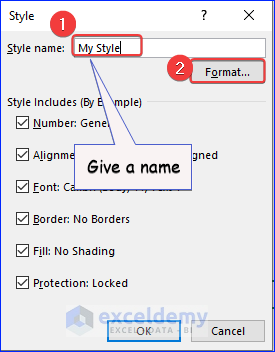
In the Style box, name your cell style and click on the Format… button.

In the Format Cells dialog box, under the Font tab, modify the Font as needed.

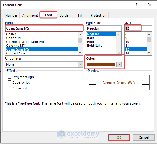
We will also change the default Fill.

Click OK twice to create the new style.
Select the whole dataset except the heading and click on Cell Styles and choose My Style.

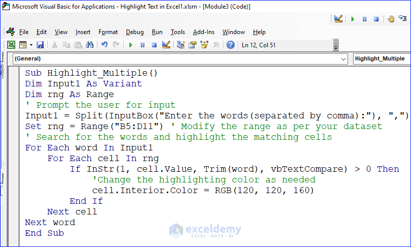
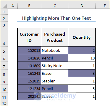
Highlight More Than One Text

Open the VBA Editor.
Copy the following code.

Sub Highlight_Multiple()
Dim Input1 As Variant
Dim rng As Range
' Prompt the user for input
Input1 = Split(InputBox("Enter the words(separated by comma):"), ",")
Set rng = Range("B5:D11") ' Modify the range as per your dataset
' Search for the words and highlight the matching cells
For Each word In Input1
    For Each cell In rng
        If InStr(1, cell.Value, Trim(word), vbTextCompare) > 0 Then
            'Change the highlighting color as needed
            cell.Interior.Color = RGB(120, 120,160)
        End If
    Next cell
Next word
End Sub

Paste the code into the editor and save it.

Go back to the Excel workbook and select the whole data table.
Press Alt + F8 together to open the Macro window.
Select the Highlight_Multiple code and hit Run.

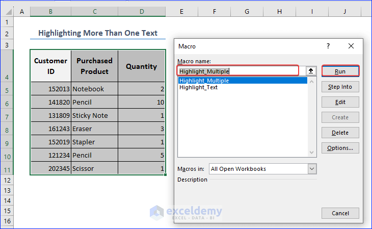
An input box will appear where you will write down the texts you want to highlight. We put “Pencil,3,2” in the box since we want to highlight it in the data table. Separate each string with a comma (without spaces).

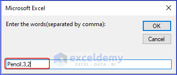
Excel has colored all the cells in the dataset that contain at least one of the chosen strings.

How Does the Code Function?

The above code is very similar to the code we used in the earlier session. We have modified that code just in 2 places.

We introduced an extra For loop in order to loop all the words that the user gives.
Instead of using the direct input, we first used the VBA Trim function to extract the words free of other delimiters like commas.

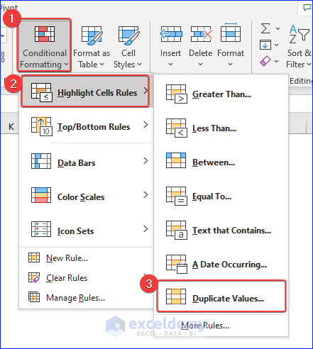
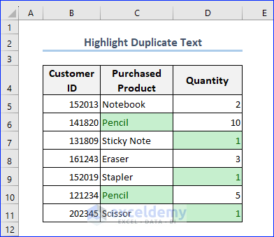
How to Highlight Duplicate Text in Excel

Select the range where you want to check for duplicates.
Under Conditional Formatting, select Highlight Cells Rules and choose Duplicate Values.

A user prompt box will appear, giving you the option to choose the format you want to apply.
Choose a format and click OK.

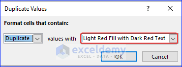
The duplicate values in your dataset are highlighted now.

Frequently Asked Questions

Does highlighting cells affect the calculation or function results in Excel?

Highlighting is just a visual formatting feature that does not impact the data or formulas.

Are there any limitations to highlighting cells in Excel?

Yes, excessive highlighting in your worksheet can impact performance. Also, the highlighting you apply to cells may not appear as expected when printing a worksheet. So, it is a good idea to preview and adjust print settings before printing to ensure accuracy.

Can I highlight cells in Excel using a formula?

Yes, you can highlight cells in Excel using a formula by applying conditional formatting.

Download the Practice Workbook

Highlighting Text.xlsm

<< Go Back to Highlight in Excel | Learn Excel

Get FREE Advanced Excel Exercises with Solutions!

12 Comments

Scot Motzny Mar 10, 2022 at 8:00 PM

Thank you for this. I was wondering if the code could be written so that it would pick up a certain number of characters after a text of string.

For example, I want it to hilight the text “Multiplier” as well as the following 7 characters. Is that possible?
- Reply
  Mrinmoy Aug 17, 2022 at 3:49 PM
  
  Hi Scot,
  The following code may fulfill your requirements.
  
  Sub TextHighlighter()
  Application.ScreenUpdating = False
  Dim Rng As Range
  Dim cFnd As String
  Dim xTmp As String
  Dim x As Long
  Dim m As Long
  Dim y, ext As Long
  cFnd = InputBox(“Enter the text string to highlight”)
  
  Color_Code = Int(InputBox(“Enter the Color Code: ” + vbNewLine + “Enter 3 for Color Red.” + vbNewLine + “Enter 5 for Color Blue.” + vbNewLine + “Enter 6 for Color Yellow.” + vbNewLine + “Enter 10 for Color Green.”))
  ext = CLng(InputBox(“Input number of additional Character to color”, , 0))
  y = Len(cFnd) + ext
  For Each Rng In Selection
  With Rng
  m = UBound(Split(Rng.Value, cFnd))
  If m > 0 Then
  xTmp = “”
  For x = 0 To m – 1
  xTmp = xTmp & Split(Rng.Value, cFnd)(x)
  .Characters(Start:=Len(xTmp) + 1, Length:=y).Font.ColorIndex = Color_Code
  xTmp = xTmp & cFnd
  Next
  End If
  End With
  Next Rng
  Application.ScreenUpdating = True
  End Sub
Gabriel Oct 28, 2022 at 2:54 AM

Hi!

Could you help me?… I´m trying to introduce a breakline in the string before cFnd.

This is the code:
xTmp = xTmp & Split(rng.Value, cFnd)(x)
.Characters(Len(xTmp) + 1, 0).Insert vbNewLine

But my problem is that I get an 1004 error with insert. Could you gave me another alternative code?
- Reply
  Sabrina Ayon Oct 31, 2022 at 12:00 PM
  Hello, GABRIEL!
  Thanks for sharing your problem with us!
  To add a new line you don’t have to write the command .Insert. You can simply use this block of the code to breakline in the string before cFnd.
```
xTmp = xTmp & Split(Rng.Value, cFnd)(x)
.Characters(Start:=Len(xTmp) + 1, Length:=y)
xTmp = xTmp & vbNewLine & cFnd
```
  To use vbNewLine, you have to make sure to do the following.
  1. After the ampersand (&) symbol, press the spacebar and get the VBA constant ‘vbNewLine‘.
  2. After the constant ‘vbNewLine‘, press one more time space bar and add the ampersand (&) symbol.
  3. After the second ampersand (&) symbol, type one more space character, and add the next line sentence in double-quotes.
  
  In VBA, there are three different (constants) to add a line break.
  vbNewLine, vbCrLf, vbLf
  
  If this is not working for you, follow the steps.
  1. Click on the character you wish to break the line from first.
  2. Then, enter a space ( ).
  3. Type an underscore (_) after that.
  4. Finally, press Enter to finish the line.
  
  Hope this will help you!
  Good Luck!
  
  Regards,
  Sabrina Ayon
  Author, ExcelDemy.
MOhamad May 6, 2023 at 1:35 PM

Hello, Thanks For 8 methods to highlight text in Excel. i Have a Problem with last method.
The code works in (English characters) But when i input for example Persian character such as (توسعه), do not Work!
- Reply
  Sourav Kundu May 8, 2023 at 5:20 PM
  
  Thank you MOhamad for your query. The Persian language is not available in the UNICODE. That’s why you are facing the problem. If you want to use the code for Persian characters, you have to modify the code slightly. The code can not take Persian language in the InputBox. So, instead of InputBox, we have to insert text to be highlighted in a cell. Let’s insert Persian text to be highlighted in the C10 cell. So, the modified vba code should be like this one.
  Sub Text_Highlighter()
  
  Application.ScreenUpdating = False
  
  Dim Rng As Range
  
  Dim cFnd As String
  
  Dim xTmp As String
  
  Dim x As Long
  
  Dim m As Long
  
  Dim y As Long
  
  cFnd = Range(“C10”).Value
  
  y = Len(cFnd)
  
  Color_Code = Int(InputBox(“Enter the Color Code: ” + vbNewLine + “Enter 3 for Color Red.” + vbNewLine + “Enter 5 for Color Blue.” + vbNewLine + “Enter 6 for Color Yellow.” + vbNewLine + “Enter 10 for Color Green.”))
  
  For Each Rng In Selection
  
  With Rng
  
  m = UBound(Split(Rng.Value, cFnd))
  
  If m > 0 Then
  
  xTmp = “”
  
  For x = 0 To m – 1
  
  xTmp = xTmp & Split(Rng.Value, cFnd)(x)
  
  .Characters(Start:=Len(xTmp) + 1, Length:=y).Font.ColorIndex = Color_Code
  
  xTmp = xTmp & cFnd
  
  Next
  
  End If
  
  End With
  
  Next Rng
  
  Application.ScreenUpdating = True
  
  End Sub
  
  You should insert your preferred cell instead of C10. And this code will highlight characters of all other languages.
  - Reply
    MOhamad May 28, 2023 at 3:52 PM
    
    Thank you for your guidance. The solution you gave worked.
    - Shamima Sultana May 29, 2023 at 12:30 PM
      
      Dear Mohamad,
      
      Thanks for your appreciation
      
      Regards
      ExcelDemy
Patrick Opiola Dec 25, 2023 at 11:30 PM

Wow! This could be one particular of the most beneficial blogs We’ve ever arrive across on this subject. Actually Wonderful. I’m also a specialist in this topic therefore I can understand your effort.
- Reply
  Shamima Sultana Dec 26, 2023 at 8:40 AM
  
  Hello Patrick Opiola,
  
  Thanks for your appreciation.
  
  Regards
  ExcelDemy
Mardell Daubney Dec 26, 2023 at 12:13 AM

I like this post, enjoyed this one appreciate it for posting. “What is a thousand years Time is short for one who thinks, endless for one who yearns.” by Alain.
- Reply
  Shamima Sultana Dec 26, 2023 at 8:38 AM
  
  Hello Mardell Daubney,
  
  Thanks for your appreciation.
  
  Regards
  ExcelDemy