Latest Posts From Mrinmoy Roy

Why Are Hidden Cells Being Pasted in Excel? When you copy and paste data in Microsoft Excel, any hidden rows and columns within the selection are also copied. ...
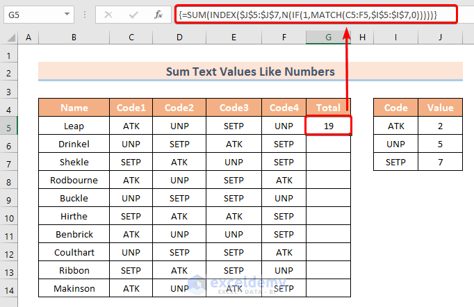
Method 1 - Using SUM, INDEX, MATCH, and IF Functions to SUM Text Values Like Numbers We have a list of names who are assigned to 4 codes individually. Each ...

Step 1 - Prepare Your Dataset Suppose we want to make of solution of Nitric Acid, Potassium Hydroxide and Water. Our target volume of the solution is 100L ...

Editing scenarios in Excel can be a great way to improve your workflow and get more out of your data. By editing scenarios in Excel, you can easily share your ...
There are two datasets below. The first one showcases daily data and the second monthly data. Step 1 - Extract the Month from the Date Create two ...

If you're looking to calculate your auto loan payment in Excel, there are a few things you'll need to know. First, you'll need to know the loan amount, the ...

In the dataset "Student Marksheet", we have columns showing student names and various courses. Next to each student's name, we have a grade for each respective ...
Method 1 - Add Precedent Arrows In cell D8, use this formula: =$D$4*C8 Cell D8 is preceded by cells D4 and C8. We can see this relation using ...
![[Fixed] Repeat Last Action Not Working in Excel (6 Solutions)](https://www.exceldemy.com/wp-content/uploads/2022/08/excel-repeat-last-action-not-working-3.png?v=1697352189)
The repeat last action feature in Excel allows users to quickly repeat the last action that they performed. This can be extremely useful when performing ...

There are many reasons you might want to move a header in Excel. Perhaps you want to change the order of the columns, or you want to move a header to a ...

What Is the Current Portion of Long-Term Debt? The Current Portion of Long-Term Debt is the amount of a company's long-term debt that is due within the ...

Method 1 - Activate Developer Tab To remove an XML mapping, activate the Developer tab first. You can only open the XML Map dialog box from the Developer tab. ...

What Is Party Ledger Reconciliation? In accounting, Party Ledger Reconciliation is the process of comparing the balances in an organization’s ledgers with the ...
The following dataset is a Product Delivery Report. We will use this dataset to generate an Excel Graph. This graph has the traditional rectangular ...

Microsoft Excel opens by default showing solid gridlines like in the following picture. Let's change the gridlines from solid to dash. Step 1 - ...
- 1
- 2
- 3
- …
- 12
- Next Page »
See Our Reviews at


Thanks for your feedback.
Hello Mr. Mejon,
Unfortunately, there is no VBA function that calculates the probability of area left to a Z score in a skewed distribution.
However, I’m suggesting you some functions that might help you.
Z.TEST function >>> Returns the one-tailed probability-value of a z-test.
KURT function >>> Returns the kurtosis of a data set.
GAUSS function >>> Returns 0.5 less than the standard normal cumulative distribution.
F.DIST.RT function >>> Returns the F probability distribution.
SKEW.P function >>> Returns the skewness of a distribution based on a population: characterization of the degree of asymmetry of a distribution around its mean.
Regards!
Hi Shabbir,
Thanks for your nice words!
Best regards.
Hi Brenda,
Follow this tutorial to fetch all the data tables from a web page. After selecting a particular data table, click on the Transform Data command to modify your data table in the Power Query Editor. There you can remove all the unnecessary columns and keep your desired data. Then hit the Close & Load button to bring the transformed data table into your worksheet.
Thanks.
Hi Anthon,
If there’s no data table on a web page, Excel will import a default document data table into the worksheet. The document table is basically a null data table.
Hi Ron,
You can see that yellow square with a red arrow in Microsoft Office Professional Plus 2016. In Excel 2019, you won’t find that because there’s no need to use the yellow box. Excel will automatically detect all the tables and make a list of ’em. All you need to do is, simply select any of the tables that you want to import and then load them directly into your Excel worksheet.
Thanks!
Hi Jennifer,
I think you have issues with your dates. Make sure your dates are accurate and in proper date format. Confirming your dates, you can apply the WEEKDAY function again. Still, if you suffer from this problem, it’s better to check the format that you’ve applied. To highlight Sunday you will apply the following formula: =WEEKDAY(B4:B12)=1. Make sure that the range inside the WEEKDAY function is legit. If everything goes just fine, this formula will highlight all the Sundays throughout your dates.
If nothing works for you, I would suggest you send your Excel file to my mail address: [email protected]. I will see what’s wrong with your data.
Thanks!
Hi KEITH,
Your problem is partly vague I think. Still, I’ve tried to build a formula that might work for you. If this doesn’t work, I would recommend you share your workbook with me or at least share a sneak peek of your dataset.
Now use this formula:
=IF(ISBLANK(K2),SUMIF(I2:I13,”asphalt field”,N2:N13),SUM(J2:J13,L2:L13))
Thanks!
Hi GVS,
This is Mrinmoy. I’m replying to you on behalf of Mr. Rifat. Currently, he has been shifted to another project. If you don’t mind, you can send your file to my email address at [email protected]. I will try to help you as much as possible.
Regards!
Hi Michelle,
You can try the following piece of code:
Sub PasteAcrossSheets()
Dim arr(3)
i = 0
For Each Worksheet In ActiveWorkbook.Sheets
Worksheet.Activate
arr(i) = ActiveSheet.Name
i = i + 1
Next
yy = ActiveWindow.RangeSelection.Address
Set xx = Application.InputBox(“Insert a range:”, “Microsoft Excel”, yy, , , , , 8)
If xx Is Nothing Then Exit Sub
mm = Application.ScreenUpdating
Application.ScreenUpdating = False
xx.Copy
Sheets(arr).Select
Range(“G5”).Select
ActiveSheet.Paste
Application.CutCopyMode = False
Application.ScreenUpdating = mm
End Sub
Hi Scot,
The following code may fulfill your requirements.
Sub TextHighlighter()
Application.ScreenUpdating = False
Dim Rng As Range
Dim cFnd As String
Dim xTmp As String
Dim x As Long
Dim m As Long
Dim y, ext As Long
cFnd = InputBox(“Enter the text string to highlight”)
Color_Code = Int(InputBox(“Enter the Color Code: ” + vbNewLine + “Enter 3 for Color Red.” + vbNewLine + “Enter 5 for Color Blue.” + vbNewLine + “Enter 6 for Color Yellow.” + vbNewLine + “Enter 10 for Color Green.”))
ext = CLng(InputBox(“Input number of additional Character to color”, , 0))
y = Len(cFnd) + ext
For Each Rng In Selection
With Rng
m = UBound(Split(Rng.Value, cFnd))
If m > 0 Then
xTmp = “”
For x = 0 To m – 1
xTmp = xTmp & Split(Rng.Value, cFnd)(x)
.Characters(Start:=Len(xTmp) + 1, Length:=y).Font.ColorIndex = Color_Code
xTmp = xTmp & cFnd
Next
End If
End With
Next Rng
Application.ScreenUpdating = True
End Sub
Hi CHRIS,
Thanks for this interesting question. It’s not about adding multiple COUNTIFS functions but multiple COUNTIF functions inside one IFS function.
Look at the following formula. It will look for two keywords “MTT” and “GL” across the text. If it finds MTT then the output will be “MTT Exists!”. For “GL” the output will be “GL Exists!”.
If nothing matches, it will return “No Results Found!”.
=IFERROR(IFS(COUNTIF(B5,”*MTT*”),”MTT Exists!”,COUNTIF(B5,”*GL*”),”GL Exists!”),”No Results Found!”)
Regards!
Hi Les,
Conditional Formatting is a static feature. Being a static feature, it doesn’t update itself automatically. However, you can apply the conditional formatting again with the default cell color to unhighlight all the completed dates.
Regards!
Hi Andrew,
It happens because of the variable types. The two variables X & Y currently have the variable type “Long” and “Integer” respectively. To get a sum value up to 2 decimal places, make both variable types “Double”. This will reserve the decimal places.
Here’s the modified code:
Function SumColoredCells(CC As Range, RR As Range)
Dim X As Double
Dim Y As Double
Y = CC.Interior.ColorIndex
For Each i In RR
If i.Interior.ColorIndex = Y Then
X = WorksheetFunction.Sum(i, X)
End If
Next i
SumColoredCells = X
End Function
I hope this will work. Regards!
Hi Joris,
The Me keyword can’t appear in a standard module because a standard module doesn’t represent an object. If you copied the code in question from a class module, you have to replace the Me keyword with the specific object or form name to preserve the original reference.
Thanks!
Hi SAM,
The first formula: =LOOKUP(2,1/($B$5:$B$12=$B$15),$C$5:$C$12) returns #N/A error for a lookup value that cannot be found. Thus, you can add the IFERROR function to tackle this issue.
For example use the following formula to return “Null” instead of #N/A error: =IFERROR(LOOKUP(2,1/($B$5:$B$12=$B$15),$C$5:$C$12),”Null”)
I hope this is what you were looking for.
Regards!
Hello Katherine,
This is a critical issue. The 4 solutions provided above are all the known solutions you will find on the internet.
So make sure, you’ve tried all the solutions accurately. Yet, you can emphasize more on solution no 2. As you described, you are facing this problem suddenly. Chances are your worksheet contains a graphic object that is invisible. So, try to find it out and remove it.
Still, if it doesn’t work properly, then you can start over with a new workbook.
Regards!
Hi Larry Kanzia,
Inverted commas can be single – ‘x’ – or double – “x”. They are also known as quotation marks, speech marks, or quotes.
You can get a single inverted comma just by pressing the comma button next to the ENTER button on your keyboard. To insert a double inverted comma, press and hold the SHIFT key, then press the comma key next to the ENTER button.
Thanks!
Hello Nicholas,
There’s no easy way to make a User-Defined Function dynamic. However, you can use an event procedure using the Worksheet_SelectionChange event to recalculate each time you change cell color. This will recalculate the formula whenever you prompt an event in your worksheet.
But I don’t recommend you to use this technique. Because it’ll slow down your workflow in Excel. Using the event procedure, the UDF will continue to calculate each time you click on your sheet.
However, you can press CTRL + ALT + F9 to recalculate manually each time you change cell color. It’s the best solution to your problem so far.
Regards!
Hello Mr. Masud,
You can easily solve your problem by combining the IF and AND functions.
Suppose, you have 3 values to compare in three cells C7, D7, and E7. For this instance, let’s say C7 is in sheet1, D7 is in sheet2, and E7 is in sheet3.
Now you are in sheet3 and you want to get a feedback (Yes or No) in cell F7.
All you need to do is, type the following formula in cell F7 of sheet3.
=IF(AND(Sheet1!C7=Sheet2!D7,Sheet2!D7=Sheet3!E7),”Yes”,”No”)
After that, press ENTER and you will get your required result.
Regards!
Hello Mr. Fazal,
You can download the attached Excel file and use that as a template.
All you need to do is input the number of years, periods per year, and balance. All the columns have their corresponding formula applied. As you provide the required information, Excel will automatically calculate the Loan Amortization Schedule for you.
Last but not the least, you have to update the variable annual interest rate (AIR) manually. If you have any lump sum amount in your consideration don’t forget to update that too!
Regards!