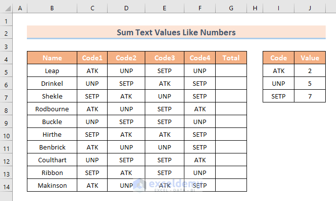
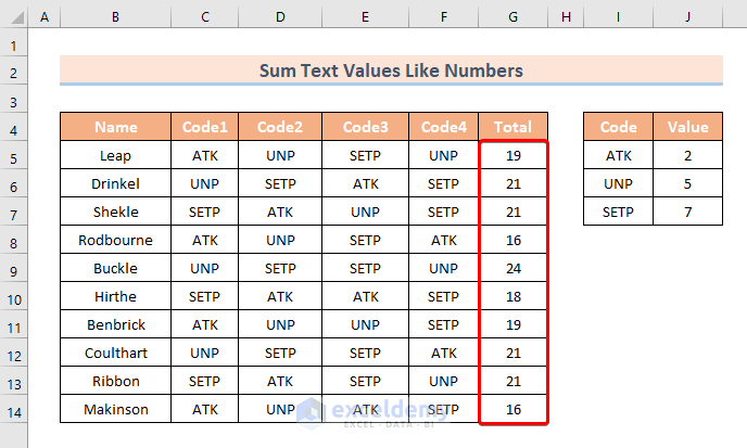
How to Sum Text Values Like Numbers in Excel (3 Methods)

Method 1 – Using SUM, INDEX, MATCH, and IF Functions to SUM Text Values Like Numbers

We have a list of names who are assigned to 4 codes individually.

Each of the assigned codes is tied to some numbers. There are 3 different codes. Each of their values is given below:

ATK = 2
UNP = 5
SETP = 7

We will write a formula to calculate the sum value of all of these codes for each person on the list.

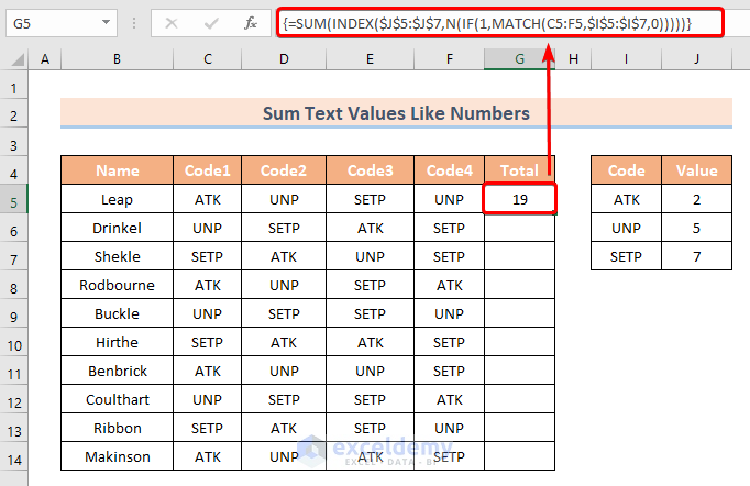
Type the following formula in cell G5. Here, G5 is the topmost cell of the column:

=SUM(INDEX($J$5:$J$7,N(IF(1,MATCH(C5:F5,$I$5:$I$7,0)))))

Press the Enter button to insert the formula into the cell if you are using Excel for Office 365. If you are using an older version of Excel, press Ctrl + Shift + Enter.

Formula Breakdown

MATCH(C5:F5,$I$5:$I$7,0): It compares the codes between the ranges C5:F5 and $I$5:$I$7. Here, the second range of writing uses the absolute cell reference because it’s fixed. It returns {1,2,3,2}. This means the codes in the range C5:F5 are equal to the codes in the range $I$5:$I$7 at the following sequence: 1,2,3, &2.
IF(1,MATCH(C5:F5,$I$5:$I$7,0)) returns {1,2,3,2}. This means the IF function multiplies 1 with the output of MATCH(C5:F5,$I$5:$I$7,0).
INDEX($J$5:$J$7,N(IF(1,MATCH(C5:F5,$I$5:$I$7,0)))): Here the INDEX function extracts the values of each of the codes from the range $J$5:$J$7. It returns {2,5,7,5}.
SUM(INDEX($J$5:$J$7,N(IF(1,MATCH(C5:F5,$I$5:$I$7,0))))): This part is equivalent to SUM({2,5,7,5}). So the SUM function adds up all the values in the array {2,5,7,5}.

Alternatively, you can use the following formula:

=SUMPRODUCT(INDEX($J$5:$J$7,N(IF(1,MATCH(C5:F5,$I$5:$I$7,0)))))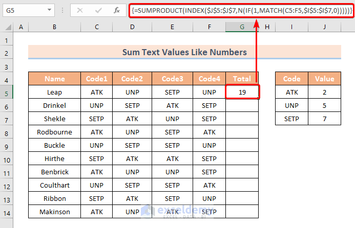

Drag down the Fill Handle in cell G5 to copy down the formula to the entire Total column.

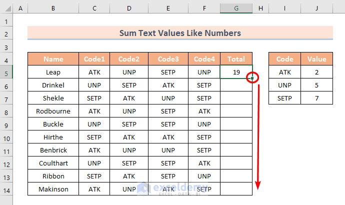
Here’s the result.

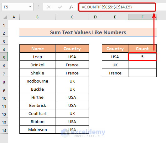
Method 2 – SUM Text Values Like Numbers Using the COUNTIF Function

In the following scenario, we have a list of names with their corresponding countries. These country names are all in text format. We will sum up the total occurrences of each of the country names.

Make a list of countries from E5 to E7.
Insert the following formula in cell F5.

=COUNTIF($C$5:$C$14,E5)

Press the Enter button.

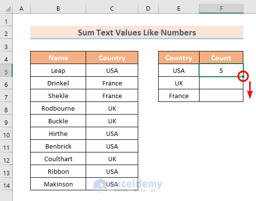
Drag the Fill Handle from cell F5 to F7 to copy down the formula.

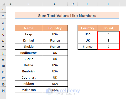
You will get the sum of the total number of occurrences of each of the country names in the column Count.

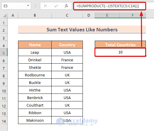
Method 3 – Combining SUMPRODUCT and ISTEXT Functions to SUM Text Values

We have a column of texts and numbers and want to ignore all the numbers and get the number of text values.

Insert the following formula in cell F5.

=SUMPRODUCT(--(ISTEXT(C5:C14)))

Press the Enter button.

This formula will sum up the number of occurrences of all the text values like numbers. In this particular case, the formula returns 10. This means the column Country has a total of 10 text values.

Formula Breakdown

ISTEXT(C5:C14): Here, the ISTEXT function varifies whether a value in the range C5:C14 is text or not. If the value is a text then it returns TRUE. Otherwise, it returns FALSE.
SUMPRODUCT(–(ISTEXT(C5:C14))): The SUMPRODUCT function adds up all the ones (1s) returned by the ISTEXT function.

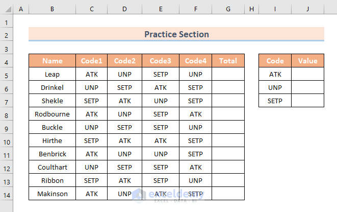
Practice Section

You will get an Excel sheet like the following screenshot at the end of the provided Excel file, where you can practice all the topics discussed in this article.